The term Bayesian statistics gets thrown around a lot these days. It’s used in social situations, games, and everyday life with baseball, poker, weather forecasts, presidential election polls, and more.

It’s used in most scientific fields to determine the results of an experiment, whether that be particle physics or drug effectiveness. It’s used in machine learning and AI to predict what news story you want to see or Netflix show to watch.

Bayesian statistics consumes our lives whether we understand it or not. So I thought I’d do a whole article working through a single example in excruciating detail to show what is meant by this term. If you understand this example, then you basically understand Bayesian statistics.

I will assume prior familiarity with Bayes’s Theorem for this article, though it’s not as crucial as you might expect if you’re willing to accept the formula as a black box.

The Example and Preliminary Observations

This is a typical example used in many textbooks on the subject. I first learned it from John Kruschke’s Doing Bayesian Data Analysis: A Tutorial Introduction with Rover a decade ago. I no longer have my copy, so any duplication of content here is accidental.

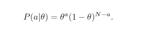
Let’s say we run an experiment of flipping a coin N times and record a 1 every time it comes up heads and a 0 every time it comes up tails. This gives us a data set. Using this data set and Bayes’ theorem, we want to figure out whether or not the coin is biased and how confident we are in that assertion.

Let’s get some technical stuff out of the way. Define θ to be the bias toward heads — the probability of landing on heads when flipping the coin.

This just means that if θ=0.5, then the coin has no bias and is perfectly fair. If θ=1, then the coin will never land on tails. If θ = 0.75, then if we flip the coin a huge number of times we will see roughly 3 out of every 4 flips lands on heads.

For notation, we’ll let y be the trait of whether or not it lands on heads or tails. This means y can only be 0 (meaning tails) or 1 (meaning heads). We can encode this information mathematically by saying P(y=1|θ)=θ.

In plain English: The probability that the coin lands on heads given that the bias towards heads is θ is θ.

Likewise, P(y=0|θ)=1 - θ.

Let’s just chain a bunch of these coin flips together now. Let a be the event of seeing a heads when flipping the coin N times (I know, the double use of a is horrifying there but the abuse makes notation easier later).

Since coin flips are independent we just multiply probabilities and hence:

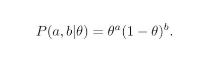
Rather than lug around the total number N and have that subtraction, normally people just let b be the number of tails and write

Let’s just do a quick sanity check with two special cases to make sure this seems right.

Suppose a,b≥ 1. Then:

• As the bias goes to zero the probability goes to zero. This is expected because we observed a heads (a≥ 1), so it is highly unlikely to be totally biased towards tails.
• Likewise, as θ gets near 1 the probability goes to 0 because we observed at least one flip landing on tails.

If your eyes have glazed over, then I encourage you to stop and really think about this to get some intuition about the notation. It only involves basic probability despite the number of variables.

The other special cases are when a=0 or b=0. In the case that b=0, we just recover that the probability of getting heads a times in a row: θᵃ.

Moving on, we haven’t quite thought of this in the correct way yet, because in our introductory example problem we have a fixed data set (the collection of heads and tails) that we want to analyze.

So from now on, we should think about a and b being fixed from the data we observed.

Bayesian Statistics

The idea now is that as θ varies through [0,1] we have a distribution P(a,b|θ). What we want to do is multiply this by the constant that makes it integrate to 1 so we can think of it as a probability distribution.

In fact, it has a name called the beta distribution (caution: the usual form is shifted from what I’m writing), so we’ll just write β(a,b) for this.

The number we multiply by is the inverse of

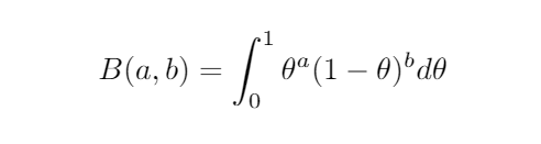
called the (shifted) beta function. Again, just ignore that if it didn’t make sense. It’s just converting a distribution to a probability distribution. I just know someone would call me on it if I didn’t mention that.

This might seem unnecessarily complicated to start thinking of this as a probability distribution in θ, but it’s actually exactly what we’re looking for. Consider the following three examples:

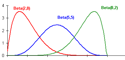
The red one says if we observe 2 heads and 8 tails, then the probability that the coin has a bias towards tails is greater. The mean happens at 0.20, but because we don’t have a lot of data, there is still a pretty high probability of the true bias lying elsewhere.

The middle one says if we observe 5 heads and 5 tails, then the most probable thing is that the bias is 0.5, but again there is still a lot of room for error. If we do a ton of trials to get enough data to be more confident in our guess, then we see something like:

Already at observing 50 heads and 50 tails we can say with 95% confidence that the true bias lies between 0.40 and 0.60.

All right, you might be objecting at this point that this is just usual statistics, where the heck is Bayes’ Theorem? You’d be right. Bayes’ Theorem comes in because we aren’t building our statistical model in a vacuum. We have prior beliefs about what the bias is.

Let’s just write down Bayes’ Theorem in this case. We want to know the probability of the bias, θ, being some number given our observations in our data. We use the “continuous form” of Bayes’ Theorem:

I’m trying to give you a feel for Bayesian statistics, so I won’t work out in detail the simplification of this. Just note that the “posterior probability” (the left-hand side of the equation), i.e. the distribution we get after taking into account our data, is the likelihood times our prior beliefs divided by the evidence.

Now, if you use that the denominator is just the definition of B(a,b) and work everything out it turns out to be another beta distribution! It’s not a hard exercise if you’re comfortable with the definitions, but if you’re willing to trust this, then you’ll see how beautiful it is to work this way.

If our prior belief is that the bias has distribution β(x,y), then if our data has aheads and b tails, we get

P(θ|a,b)=β(a+x, b+y).

The way we update our beliefs based on evidence in this model is incredibly simple!

Now I want to sanity check that this makes sense again. Suppose we have absolutely no idea what the bias is. It would be reasonable to make our prior belief β(0,0), the flat line. In other words, we believe ahead of time that all biases are equally likely.

Now we run an experiment and flip 4 times. We observe 3 heads and 1 tails. Bayesian analysis tells us that our new (posterior probability) distribution is β(3,1):

Yikes! We don’t have a lot of certainty, but it looks like the bias is heavily towards heads.

Danger: This is because we used a terrible prior. In the real world, it isn’t reasonable to think that a bias of 0.99 is just as likely as 0.45.

Let’s see what happens if we use just an ever so slightly more modest prior. We’ll use β(2,2). This assumes the bias is most likely close to 0.5, but it is still very open to whatever the data suggests.

In this case, our 3 heads and 1 tails tells us our updated belief is β(5,3):

Ah. Much better. We see a slight bias coming from the fact that we observed 3 heads and 1 tails. This data can’t totally be ignored, but our prior belief tames how much we let this sway our new beliefs.

This is what makes Bayesian statistics so great! If we have tons of prior evidence of a hypothesis, then observing a few outliers shouldn’t make us change our minds.

On the other hand, the setup allows us to change our minds, even if we are 99% certain about something — as long as sufficient evidence is given. This is just a mathematical formalization of the mantra: extraordinary claims require extraordinary evidence.

Not only would a ton of evidence be able to persuade us that the coin bias is 0.90, but we should need a ton of evidence. This is part of the shortcomings of non-Bayesian analysis. It would be much easier to become convinced of such a bias if we didn’t have a lot of data and we accidentally sampled some outliers.

Now you should have an idea of how Bayesian statistics works. In fact, if you understood this example, then most of the rest is just adding parameters and using other distributions, so you actually have a really good idea of what is meant by that term now.

Drawing Conclusions

The main thing left to explain is what to do with all of this. How do we draw conclusions after running this analysis on our data?

You’ve probably often heard people who do statistics talk about “95% confidence.” Confidence intervals are used in every Statistics 101 class. We’ll need to figure out the corresponding concept for Bayesian statistics.

The standard phrase is something called the highest density interval (HDI). The 95% HDI just means that it is an interval for which the area under the distribution is 0.95 (i.e. an interval spanning 95% of the distribution) such that every point in the interval has a higher probability than any point outside of the interval:

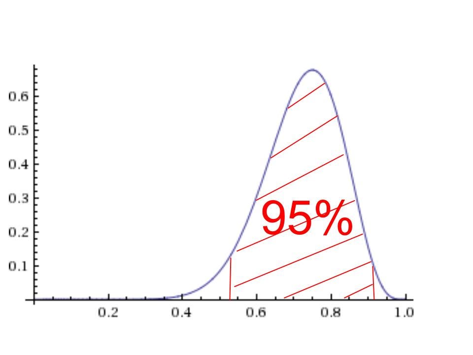
(It doesn’t look like it, but that is supposed to be perfectly symmetrical.)

The first is the correct way to make the interval. Notice all points on the curve over the shaded region are higher up (i.e. more probable) than points on the curve not in the region.

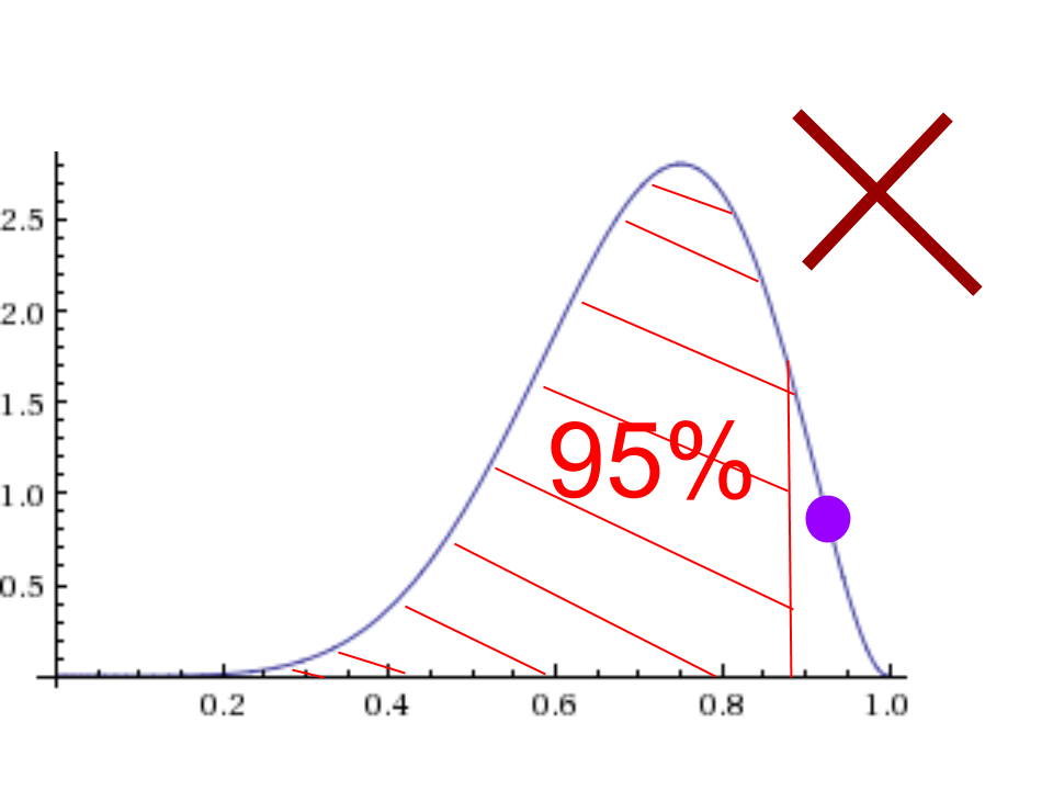
Note: There are lots of 95% intervals that are not HDI’s. The second picture is an example of such a thing because even though the area under the curve is 0.95, the big purple point is not in the interval but is higher up than some of the points off to the left which are included in the interval.

Lastly, we will say that a hypothesized bias θ₀ is credible if some small neighborhood of that value lies completely inside our 95% HDI. That small threshold is sometimes called the region of practical equivalence (ROPE) and is just a value we must set.

If we set it to be 0.02, then we would say that the coin being fair is a credible hypothesis if the whole interval from 0.48 to 0.52 is inside the 95% HDI.

A note ahead of time, calculating the HDI for the beta distribution is actually kind of a mess because of the nature of the function. There is no closed-form solution, so usually, you can just look these things up in a table or approximate it somehow.

Both the mean μ=a/(a+b) and the standard deviation

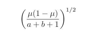
do have closed forms.

Thus I’m going to approximate for the sake of this article using the “two standard deviations” rule that says that two standard deviations on either side of the mean is roughly 95%.

Caution, if the distribution is highly skewed, for example, β(3,25) or something, then this approximation will actually be way off.

Let’s go back to the same examples from before and add in this new terminology to see how it works. Suppose we have absolutely no idea what the bias is and we make our prior belief β(0,0), the flat line.

This says that we believe ahead of time that all biases are equally likely. Now we do an experiment and observe 3 heads and 1 tails. Bayesian analysis tells us that our new distribution is β(3,1).

The 95% HDI in this case is approximately 0.49 to 0.84. Thus we can say with 95% certainty that the true bias is in this region. Note that it is not a credible hypothesis to guess that the coin is fair (bias of 0.5) because the interval [0.48, 0.52] is not completely within the HDI.

This example really illustrates how choosing different thresholds can matter, because if we picked an interval of 0.01 rather than 0.02, then the hypothesis that the coin is fair would be credible (because [0.49, 0.51] is completely within the HDI).

Let’s see what happens if we use just an ever so slightly more reasonable prior. We’ll use β(2,2). This gives us a starting assumption that the coin is probably fair, but it is still very open to whatever the data suggests.

In this case, our 3 heads and 1 tails tells us our posterior distribution is β(5,3). The 95% HDI is 0.45 to 0.75. Using the same data we get a little bit more narrow of an interval here, but more importantly, we feel much more comfortable with the claim that the coin is fair. It is a credible hypothesis.

This brings up a sort of “statistical uncertainty principle.” If we want a ton of certainty, then it forces our interval to get wider and wider. This makes intuitive sense, because if I want to give you a range that I’m 99.9999999% certain the true bias is in, then I better give you practically every possibility.

If I want to pinpoint a precise spot for the bias, then I have to give up certainty (unless you’re in an extreme situation where the distribution is a really sharp spike). You’ll end up with something like: I can say with 1% certainty that the true bias is between 0.59999999 and 0.6000000001.

We’ve locked onto a small range, but we’ve given up certainty. Note the similarity to the Heisenberg uncertainty principle which says the more precisely you know the momentum or position of a particle the less precisely you know the other.

Mathematical Uncertainty PrinciplesHow to understand a core idea from Quantum Mechanics.medium.com

Summary

Let’s wrap up by trying to pinpoint exactly where we needed to make choices for this statistical model. The most common objection to Bayesian models is that you can subjectively pick a prior to rig the model to get any answer you want.

In the abstract, that objection is essentially correct, but in real life practice, you cannot get away with this.

Here’s a summary of the above process of how to do Bayesian statistics.

Step 1 was to write down the likelihood function P(θ | a,b). In our case this was β(a,b) and was derived directly from the type of data we were collecting. This was not a choice we got to make.

Step 2 was to determine our prior distribution. This was a choice, but a constrained one. In real life statistics, you will probably have a lot of prior information that will go into this choice.

Recall that the prior encodes both what we believe is likely to be true and how confident we are in that belief. Suppose you make a model to predict who will win an election based on polling data. You have previous year’s data and that collected data has been tested, so you know how accurate it was!

Thus forming your prior based on this information is a well-informed choice. Just because a choice is involved here doesn’t mean you can arbitrarily pick any prior you want to get any conclusion you want.

I can’t reiterate this enough. In our example, if you pick a prior of β(100,1) with no reason to expect to coin is biased, then we have every right to reject your model as useless.

Your prior must be informed and must be justified. If you can’t justify your prior, then you probably don’t have a good model. The choice of prior is a feature, not a bug. If a Bayesian model turns out to be much more accurate than all other models, then it probably came from the fact that prior knowledge was not being ignored.

It is frustrating to see opponents of Bayesian statistics use the “arbitrariness of the prior” as a failure when it is exactly the opposite. On the other hand, people should be more upfront in scientific papers about their priors so that any unnecessary bias can be caught.

Step 3 is to set a ROPE to determine whether or not a particular hypothesis is credible. This merely rules out considering something right on the edge of the 95% HDI from being a credible guess.

Admittedly, this step really is pretty arbitrary, but every statistical model has this problem. It isn’t unique to Bayesian statistics, and it isn’t typically a problem in real life. If something is so close to being outside of your HDI, then you’ll probably want more data.

For example, if you are a scientist, then you re-run the experiment or you honestly admit that it seems possible to go either way.