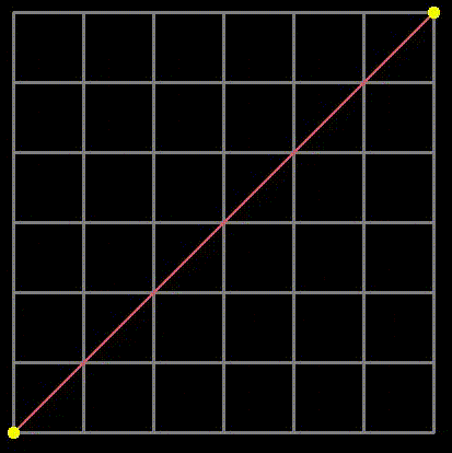
In this essay, we’re going to obsess about paths on a two-dimensional grid. Here is what such a path might look like:

We’ll think about counting paths that satisfy certain properties.Even though the simple joy of counting things should be motivation enough, I’ll provide some additional practical reasons you should care. How many times have you seen a graph with an x and y-axis? For example, the graph of the price of a stock, with the x-axis being time and y being the stock price. In other words, time series. Many successful mathematical models think of these paths as grids which the stock price or whatever quantity is being plotted traverse. At each step, the price can go up or down. Motion that follows these rules is called “Brownian motion”, first used to describe the random motion of dust particles. Another analogy is a gambler who tosses a coin, winning $1 on heads and losing $1 on tails. The paths on the grid drawn above represent his total profit for some sequence of heads and tails. Hence, the paths are called “gambler paths”.

These kinds of models then helps with pricing investment tools built on these stocks (like options, etc.).

We’ll first consider the simplest case of square grids. The total number of paths where you can only move towards your target, never away from it (so only up or right steps in figure 1 above) is high school Math. Then there is a famous sequence called the Catalan numbers which define the paths which do this without crossing the main diagonal (red line in figure 1). Notice the path shown in figure 1 actually does cross it twice and hence is “invalid” under these constraints.

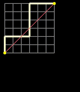
Taking Theodore Sturgeon's advice and “asking the next question”, we’ll consider paths on rectangular grids (generalizing square ones). This is related closely to “Bertrand’s ballot problem” (candidate A gets p votes, candidate B gets q votes, what is the probability candidate A was always in the lead after every vote). And finally, we’ll go back to square grids, but consider paths that cross the main diagonal k times instead of not crossing it at all. When k=0, we should recover the original sequence, of course. The final question is doing both generalizations together — paths that move on a rectangular grid, crossing some horizontal line k times. But with the tools we’d have developed by then, the solution to this one will just pop out very naturally.

1. Total Paths

Let’s start really easy and consider the total paths from the bottom left of the grid to the top right that only move right or up in the square grid of figure 1. When the grid is n×n, we know we have to take a total of 2n steps, n of them towards the right and n upwards. It just becomes a matter of choosing which n of those 2n steps will be a move upwards and which will be a move to the right. Hence, the total such paths becomes {2n \choose n}.

2. Dyck Paths

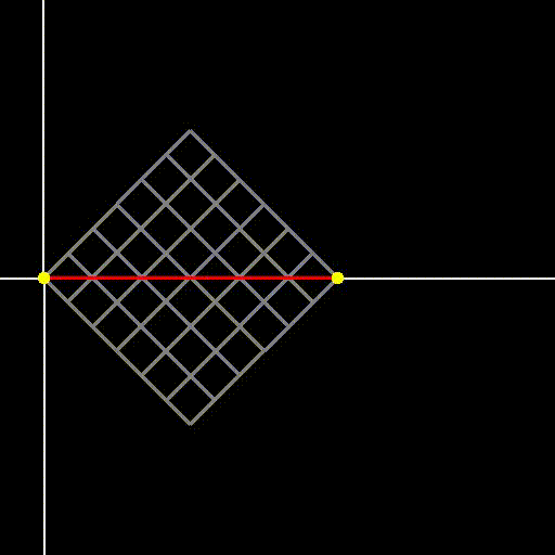
We alluded in the beginning to paths on the grid being useful for modeling time-series (like stock prices). This was furnished by considering dividing time into a discrete grid with the stock price going either up one unit or down one unit at each time point on the grid. It’s not immediately clear how the path in figure 1 might be related to this. But, it becomes obvious once we rotate it like figure 2 does below.

The kinds of paths we’ll first think about are ones that start and end at y=0 (two yellow points in figure 3 below) and avoid crossing the central red line of figure 2. These are called “Dyck paths”. They either stay above or below the x-axis. For every path that stays above, there is a symmetric path that stays below and vice versa as we can see by reflecting them as in figure 3 below.

Notice that since we start and end at y=0, we must take as many up steps as down steps. So, the total number of steps must be even, say 2n. Here, n is the side of the square grid.

Let’s say the number of such paths that stay below y=0 (like the orange path in figure 3) in a grid with side n is c_n. In our analogy of the gambler tossing a coin, this represents starting and ending at 0$ without ever having a positive balance (or equivalently, ever having a negative balance).

We’ll calculate c_n in two ways.

2.1 Andre’s Reflection Method

We know there are {2n \choose n} total paths but we want to exclude the ones that cross the main diagonal (purple line in figure 4 below). Now, note that any path that crosses the purple line from below it to above necessarily touches the orange line right above the purple line. This makes identifying the undesirable paths easier since the purple line is touched at least when we’re at the start and end of any of our paths (desirable or otherwise) and might be touched without crossing more times in some of them. The orange line on the other hand, is touched only for the undesirable paths, making for a cleaner identifying criterion.

Now comes the key insight. Consider any path that touches the orange line, at some point, and then goes on to the point where all paths end (in figure 4, this is the red point). Such a path is by definition an undesirable path we want to exclude. Now, split this path into two segments. The first segment goes from the blue point, where all paths start to the orange line. The second segment then goes from there to the red end-point. Now, reflect the first segment about the orange line. The reflection is unique for each sub-path leading up to the orange line. Also, the reflected paths happen to form another rectangular grid. As can be seen in figure 4, this new grid shown in bright-yellow has one less column and one more row than the original (so, n+1 down steps and n up steps.

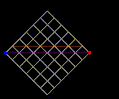
Now, since each undesirable path on the original grid maps to a path on the bright yellow grid, we can count the undesirable paths. Since we still have to take a total of 2n steps for paths on the bright yellow grid, but n-1 up-steps, the total paths is the number of ways of choosing which of the 2n steps will go upwards (with the rest going downwards). Hence, the undesirable paths become {2n choose n-1}. And with this, we can find the desirable paths (ones that don’t touch the main diagonal) as the total paths ({2n choose n}) subtracted by the undesirable paths. We hence get the total paths that go from (0,0) to (n,n) on the grid with n up-steps and n down-steps without crossing the main diagonal, c_n:

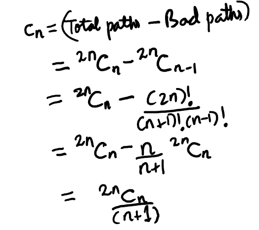
Note that the total paths on the grid was {2n \choose n} and the number of paths that stay at or below the main diagonal are 1/(n+1) of them.

2.2 Using a Recurrence

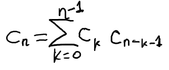
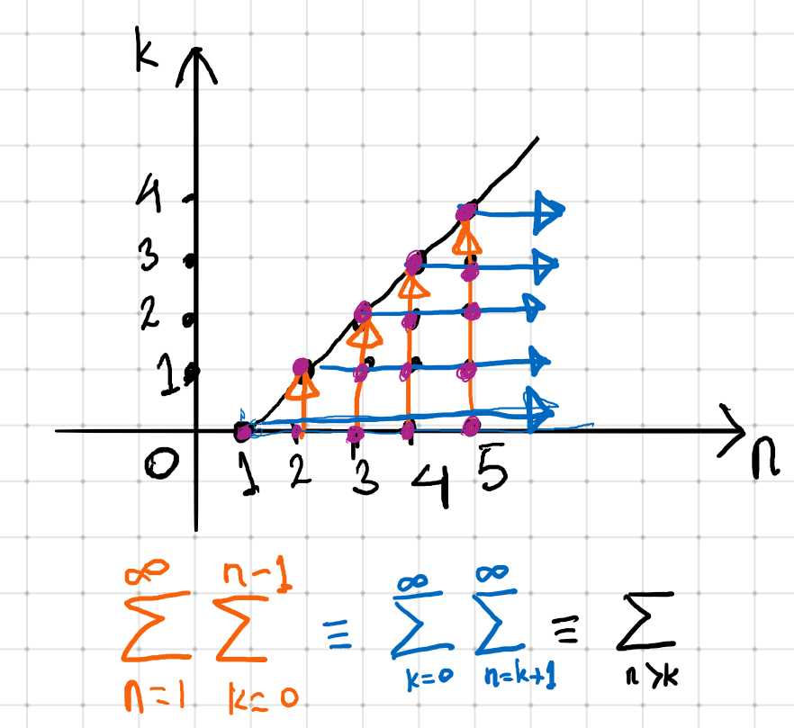
Now, we’ll take a path involving less pictures, but one that will ultimately lead to a powerful tool that can help solve a whole family of these “paths on a grid” problems. This tool is the “generating function” of a sequence. First, let’s form a recurrence. Think of the number of paths that first touch the main diagonal (or x-axis) at a certain number of steps after the starting point.

1. If they are not to touch it before this, we must first take a step upwards and reach the orange line in figure 5 below.
2. After that, we take 2k steps in a way that we don’t go below the orange line again, beginning and ending at it. The number of ways of taking these 2k steps is c_k by definition.
3. Finally, we take a step downwards and get back to the main diagonal (or x-axis).
4. So far, we have taken one step up, 2k steps on the orange path and one step down, so 2k+2 steps. This means we’re left with 2n-2k-2 steps. We now take these steps without violating the original condition, hence staying above the x-axis. The number of ways of doing this is c_{n-k-1} by definition.

So, if the orange path is of length 2k, we first touch the main diagonal (or x-axis) at step 2k+2. The total paths that touch the main diagonal after 2k+2 steps and satisfy the original condition of staying above the main diagonal becomes: c_k ×c_{n-k-1}. Now, the orange segment in figure 5 can take any length from 0 to 2(n-1), corresponding to k going from 0 to n-1. Here, the paths that correspond to k=0 and k=n-1 never touch the x-axis (or main diagonal) except at the beginning and end of their journeys. Hence, we get the recurrence:

This is the same recurrence as in exercise 12–4 of the book “Introduction to Algorithms” by Cormen et.al. which is considered the bible of Computer Science (if a recruiter from Google reaches out to you, they will recommend this book). That chapter however, deals with binary trees (an important data structure in CS that allows for many operations like look-up, insertion, deletion, etc. all in O(log(n)) steps). Why would they include a recurrence about paths on a grid in a chapter on binary trees? Well actually, it is meant to describe the number of binary trees with one node reserved for the root and all nodes having zero or two children. It is easy to see that it’ll be satisfied in that context since we reserve one node for the root, assign k of the nodes to the left sub-tree and the remaining n-k-1 nodes to the right sub-tree.

And since the fact that they satisfy the same recurrence with the same starting conditions must mean that the sequences themselves are the same, we see that the number of paths on a grid where we take n steps up and n down without crossing the main diagonal is equivalent to the number of binary trees with n nodes (both sequences denoted by the Catalan numbers). If you read the Wikipedia article on Catalan numbers, you’ll see that there are many other seemingly unrelated counting problems that are all governed by this sequence.

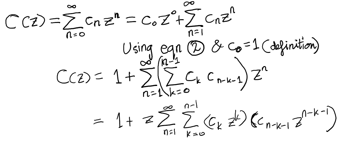
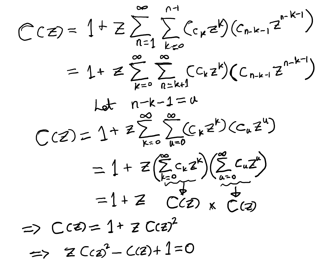
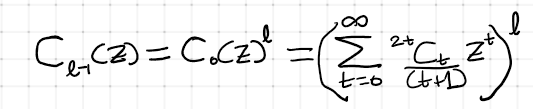
Mapping to other sequences is all well and good, but can we use the recurrence above to actually get the closed-form solution in equation (1)? To do this, we first define the generating function of the sequence, c_n by taking the terms and incorporating them into an infinitely large polynomial:

If we can find C(z) in closed form, it might help us get the expression for c_n by asking what the coefficient of z^n would have been if we expressed it as a polynomial. Let’s plug the recurrence from equation (2) into the generating function we defined above.

Now, we can simplify the double summation over n and k in the equation above by flipping the roles of n and k. In the figure below, we basically want to sum the value of the summand over all the purple points. The summation in the equation above goes to each n and sums over possible values of k that are less than or equal to the corresponding n. This is equivalent to going in the direction of the orange arrows in figure 6 below.

Equivalently, we can sum first over k and then consider the values of n for each k. This corresponds to summing over the blue arrows in figure 6 below. Both strategies capture all the purple points we want to capture. Hence, flipping the summations is possible as shown at the bottom of figure 6.

Now, when we flip the summations so that we sum over k first, the two variables separate out nicely as shown in the blurb below. In the end, we’re able to separate the summations out and get a quadratic equation in terms of C(z) and z.

This equation can be solved for C(z) by using the quadratic formula to get:

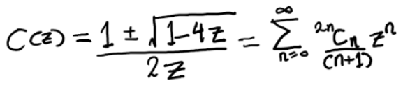
We know that C(0)=1 but this is only possible when we consider the negative sign in the two solutions expressed in equation (5) above.

And finally, we can expand the right hand side using either the generalized binomial theorem or Taylor series to get the same expression for c_n as we got in equation (1).

3. Raising the Glass Ceiling

3.1 Generalizing the Sequence of Paths

The Dyck paths we considered in section 2 always started and ended at the same level (taken to be level 0). Real life paths on a grid won’t necessarily satisfy this constraint. A real gambler could choose to stop tossing the coin at a certain level of profit or loss. Let’s take the grid we’ve been working with and lift the target from ending back at 0 to ending at a (for example) 4$ profit for the gambler (orange line).

We still start at the blue point and end up at the red point, but now the red point can be at a different vertical level than the blue one. How many paths go from the blue point to the red point without crossing the orange line? In other words, how many ways can the gambler reach 4$ after 8 heads and 4 tails without ever crossing 4$? Note first that this is equivalent to the number of paths where his balance never goes negative (paths where he never crosses the purple line representing 0$ balance in figure 6 from above). This can be seen by starting with a path that crosses the orange line and then rotating the entire grid, hence reversing the path. This then becomes a path where the balance goes negative.

Now, let’s find the number of paths.

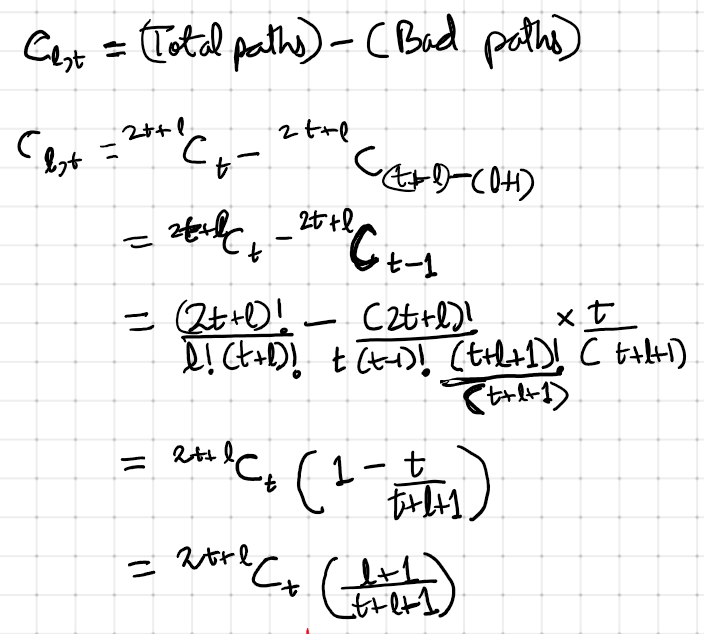
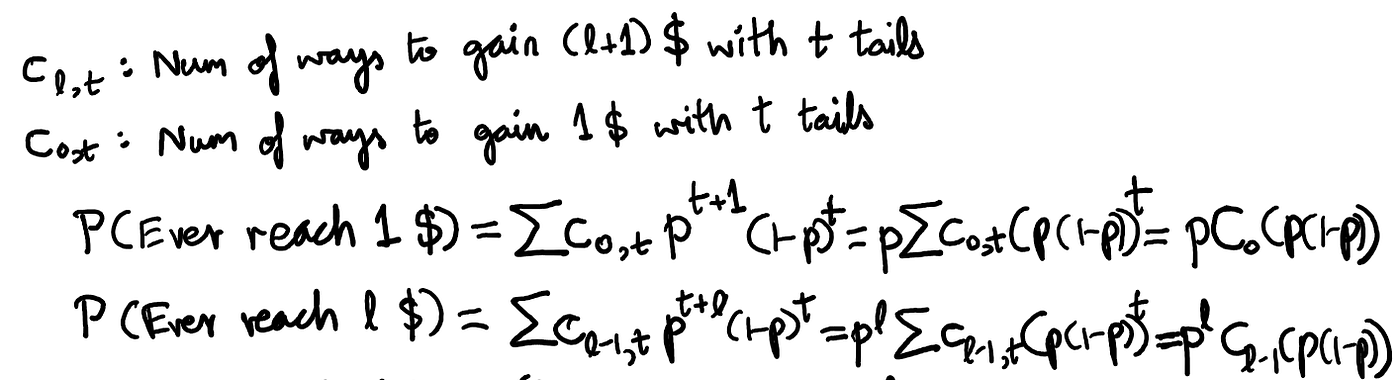
Definition-1: Let c_{l,t} be the number of paths where a gambler gets t tails and t+l heads, reaching a profit of l$ without ever crossing l$.

3.2 The Reflection Method Again

We can use Andre’s reflection method like before, employing the same technique as we did in figure 4. Figure 8 below is another GIF demonstrating what the process looks like when we want to go from the blue point to the red point without crossing the orange line. If you’re not sure what’s going on, just re-visit section 2.1.

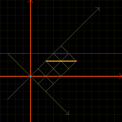
Figure 8.1 below provides a static view of the reflection method. It involves:

1. Reflect the origin (blue point) about the purple line (y=l+1). The purple line is the level we can never touch.
2. Draw the yellow grid from the reflected blue point to the red point. This grid represents the “bad paths” we want to exclude.
3. Notice that the height of the yellow grid is (t-1).

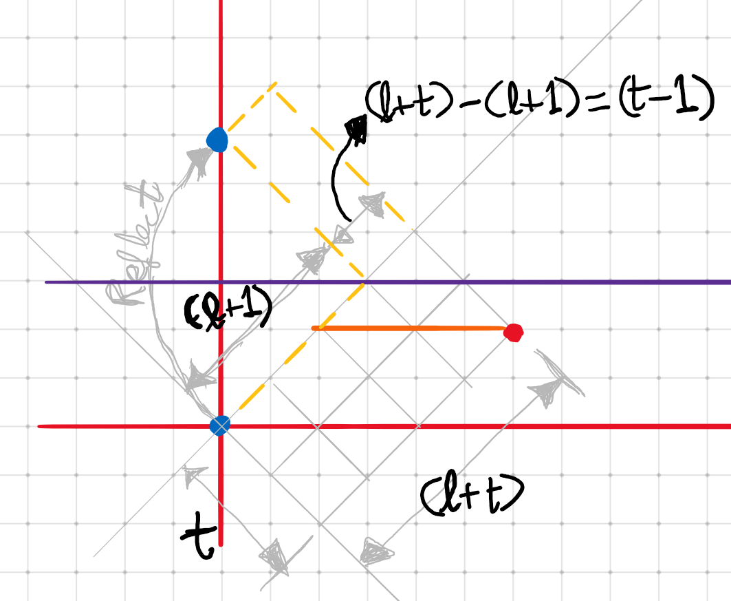
Now, we know that the gambler needs (t+l) heads and t tails, making the total paths {2t+l \choose t}. Since the total steps required in the yellow grid formed after reflection doesn’t change, we can get the paths of interest:

4.3 Generating Functions

Now, we’ll get the actual closed-form expression for c_{l,t} using generating functions. If we were only worries about finding c_{l,t}, the reflection method approach is frankly, much simpler. But, the generating function will give us a framework for solving a more generalized version of the problem.

An alternate definition will make our job a lot simpler:

Definition-2: c_{l,t} is also the number of ways of reaching (l+1)$ with t heads and t+l+1 tails for the first time.

Notice in the second definition, we aren’t allowed to touch the target (l+1)$ level before finally reaching it while in the first, we are allowed to touch l$, just not cross it. The two are equivalent since once we reach l$ in t tails and t+l heads, there is only one way to get to (l+1)$ in one more toss, which is to get another heads and earn another dollar.

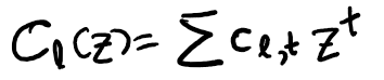
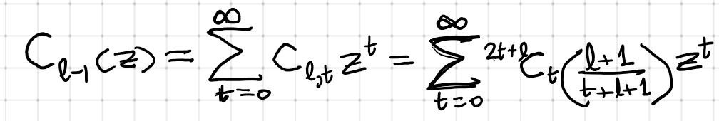
Now, define the generating function for the sequence that defines the ways in which the gambler reaches l$:

4.3.1 Consolidating the Generating Functions

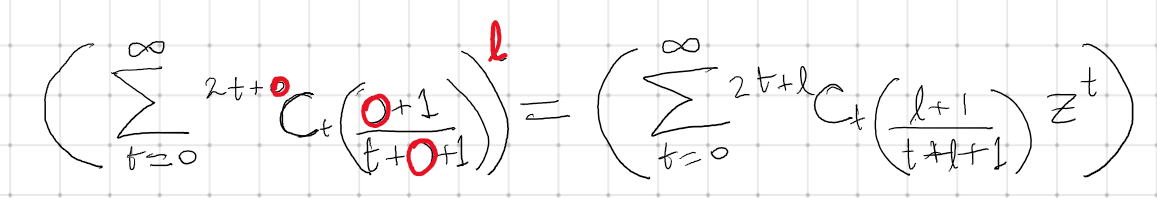
Note that if we plug l=0 in equation (6) above, we get the C_0(z)=C(z) defined in defined in equation (3) and solved for in equation (5). Can we express the other C_l(z)’s in terms of C(z) as well?

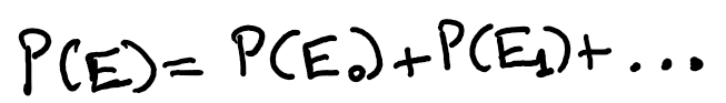
We use a nifty probability trick to do this. Here, definition 2 of c_{l,t} comes in handy. Consider the gambler tossing a coin non-stop until he reaches 1$. What is the probability that he will ever reach his target 1$? Define that as event E. Now, define E_t as the event that he reaches 1$ for the first time with exactly t tails (so he must have (t+1) heads by then). So, E happens if he either reaches 1$ for the first time with 0 tails (just gets a heads in the first toss) OR reaches 1$ with 1 tail OR with 2 tails and so on:

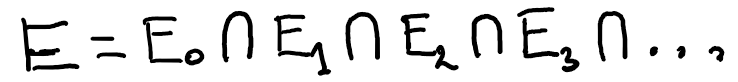
Now, each of E_0, E_1,.. are mutually exclusive events (only one of them can be true at a time). So, the probability of event E becomes:

Now, what is (for example) P(E_2)? It’s the number of ways of getting to 1$ with 2 tails and 3 heads for the first time on toss 5, multiplied by the probability of 2 tails multiplied by the probability of 3 heads. We insist on counting paths where he reaches 1$ for the first time with 2 tails because if he reached 1$ sooner, (say with just one tail), he would have stopped there and not really reached 1$ with 2 tails, which is what E_2 is describing. We can repeat this argument for reaching l$ (instead of 1$) and get the following relationship of these probabilities in terms of the generating functions defined in equation (6) (here, p is the probability of the coin he’s tossing coming up heads).

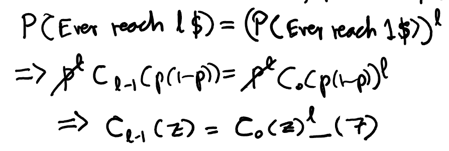
Now, think of a gambler who is targeting l$. At some point, he has to increase his fortune by 1$. And once he does that, we can imagine he puts this 1$ in his bank so his earnings are back to 0$ and now he’s targeting (l-1)$. But now, he simply has to get to 1$ again as if he were starting from scratch because the coin he’s tossing doesn’t care about his history. So, he has to repeat the feat of reaching 1$ and putting it in his bank l times. But each time he wants to reach 1$, its as if the game resets and so, the probability of this happening remains the same. Hence, the probability:

P(gambler will reach l $)=P(gambler will reach 1$)×P(gambler will reach 1$)… (ltimes).

Using this and equation (6.5), we get a relationship between the generating functions:

4.3.2 Defining a Recurrence

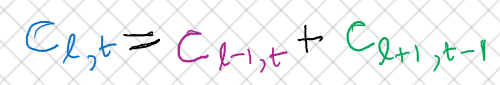
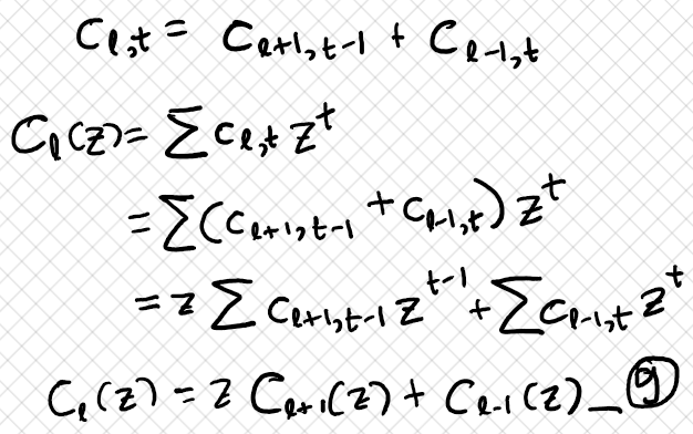
Now, we can define a recurrence for the c_{l,t} terms by thinking of the first coin toss the gambler makes. Refer to figure 9 below. Initially, the gambler is at the blue point and seeks to reach the red point, which is at level l with t tails. If his first toss is a heads, he reaches the purple level. Here, he has to climb (l-1) levels to get to the red point, but still with t tails. If he tosses a tails on the first toss, he reaches the green level where now he has to climb (l+1) levels to reach the red point. And, he now has to toss one less tails in order to reach the red point.

Hence, we get the recurrence:

4.3.3 Solving the Recurrence

Now, we can use equation (8) to translate the recurrence for the paths, c_{l,t} into a recurrence for the generating function: C_{l}(z).

And now, the relationship devised from the probability trick of equation (7) comes in handy:

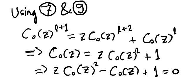
We see that this has led us to the same expression as equation (4). And the solution to this (from simply solving the quadratic equation in C_0(z)=C(z)) is the one given in equation (5).

We already knew the expression for C_0(z) and hence, c_{0,t}. What we need is an expression for c_{l,t}. Let’s start with

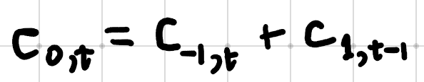
Now, c_{-1,t}=0 since by definition-2, it represents the number of ways for the gambler to hit 0$ for the first time with t tails. But since he starts with 0$, the end of his path won’t be the first time he hits 0$. Hence, the number of ways to do this is 0. So, c_{1,t-1}=c_{0,t}. Substituting t=t+1, c_{1,t}=c_{0,t+1}. Now that we have c_{1,t} and c_{0,t}, we can use them to find c_{2,t} from equation (8). And continue this process to finally get to c_{l,t}.

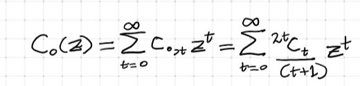
But, we have a closed-form from equation 5.5, so why bother with this iterative approach. What we do get is a very beautiful identity when we plug in the generating functions. From equation (1) and the definition of the generating function we get:

And using equation (7) we derived with our probability trick:

Using the result of equation (5) we have:

Equating the right hand sides of equations (12) and (13), we get this incredible identity also covered in example 5 of section 7.5 of the book “Concrete Mathematics” by Graham, Knuth and Patashnik. Notice how the l on the left hand side simply marches in and replaces the 0’s. This identity has more than an aesthetic appeal we’ll use it in the next section to solve yet another generalization. See here for a discussion on this identity.

5. Multiple Crossings

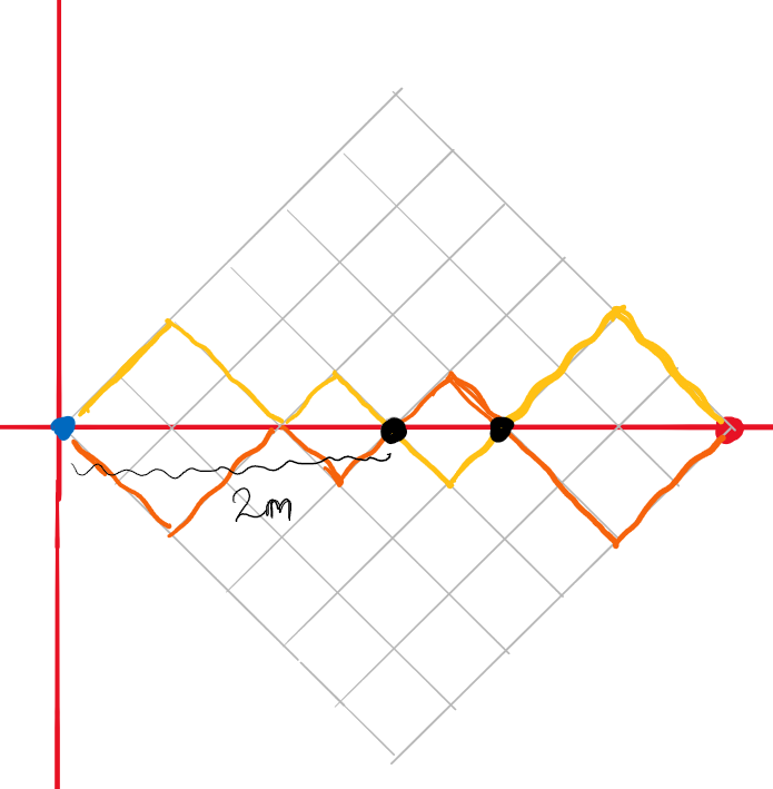
In section 2, we considered paths that begin and end at level 0, crossing it exactly 0 times. In section 3, we generalized to paths that start at level 0, but end at level l. Now, let’s generalize them in a different direction. Consider paths that start and end at level 0; and cross the main diagonal exactly k times. When k=0, we obviously get back the Dyck paths from section 2. Figure 10 below shows a yellow path on a grid with t=5 that crosses the main diagonal at the two black points. The orange path is a reflection of the yellow path and also crosses the main diagonal the same number of times, from the opposite sides.

To make things concrete, consider a gambler who starts and ends at a fortune of 0$, getting t heads and t tails. We saw that the total number of paths is {2t \choose t} and the number of paths that don’t cross 0$ are 2 c_t = 2{2t\choose t}/(t+1) — the same as equation (1) apart from the factor of 2 which accounts for paths that stay at or above or at or below the 0$ mark (two such symmetric paths are shown in figure 3).

We now want to find paths that start and end at the 0$ mark, but cross the 0$ line exactly k times. Let’s call the number of such paths r_{k,t}. Obviously, we have r_{0,t}=2 c_t (for c_t defined in equation (1)).

4 .1 A Recurrence

First, we can get a recurrence for the r_{k,t} terms by considering the first place in the path where it crosses the x-axis. This is section 1 of his journey and let’s say it happens on 2m tosses (it has to be even since the gambler has to get an equal number of heads and tails). The number of ways to do this is just c_m.

From here, section 2 of the gamblers journey starts and he has (2t-2m) tosses left and needs to cross the main diagonal another (k-1) times to satisfy the condition. The number of ways to do this is by definition, r_{k-1,t-m}.

The total ways of completing his journey is the number of ways of completing section 1 times the number of ways of completing section 2. But that would imply paths that cross the x-axis after m tails. For the total paths, m can be anything from 1 to n-1. So, we sum over all these possibilities to get:

4.2 The Generating Function

Like before, let’s define the generating function, R_{k}(z):

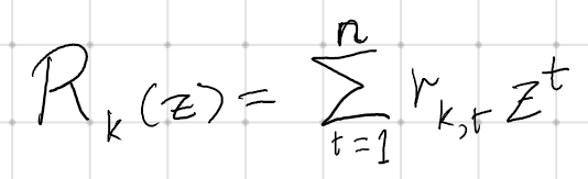
Notice that we start now at t=1 unlike for the generating function, C_l(z). This is because r_{k,0}=0 (0 tails means 0 heads as well and if we have no tosses, how can we cross the main diagonal k times).

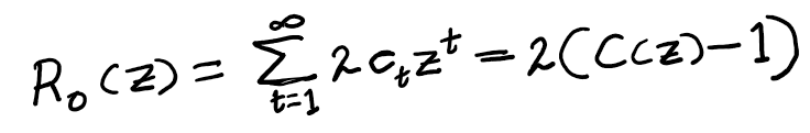
The case where we cross the main diagonal k=0 times is just the paths we’ve seen before and the generating function for that case should be simple:

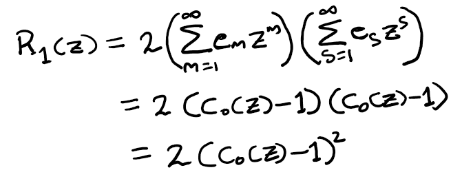
Now, let’s extend this to k=1. We get (using our observation the recurrence in equation (14)):

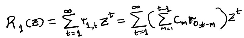
Now, we can use the fact that r_{0,t}=2c_t as discussed earlier along with the summation index-switching trick we used in equation (4) and figure 6 to get:

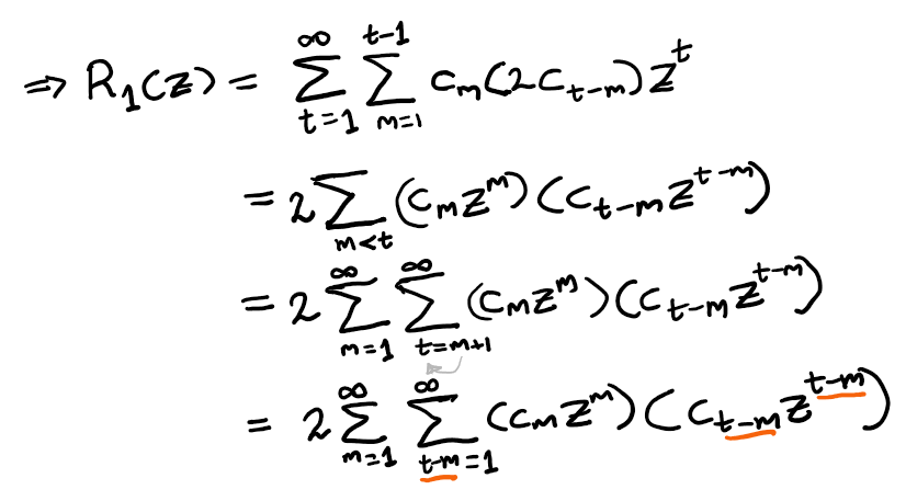
Now, re-index t-m=s and use the result of equation (13) to separate the summations and express in terms of generating functions seen before:

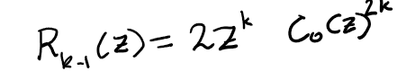
We can repeat this whole process k-1 times to get:

From equation (10) where we got a relationship for C_0(z) we have:

Substituting into equation (15) gives us:

And from equation (14):

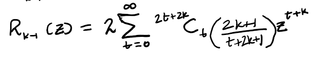
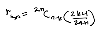
But we want the coefficient of z^t. So, we let n=t+k, meaning t=n-k. This gives us the expression for the generating function:

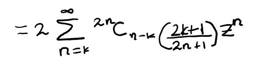
Implying:

Note that r_{k,n}=0 if n<k which makes sense; how can you cross the diagonal ktimes if your path length isn’t long enough? The Math presented is taken from here.

6. Next Questions

We should never cease to stop asking the next question. Here are some further generalizations, all of which have nice expressions:

1. The number of paths that stay below some arbitrary level.
2. The number of paths that stay between two levels.
3. The number of paths that cross some arbitrary level k times.