The knowledge of which geometry aims is the knowledge of the eternal. — Plato

Inphysics, most of the time we need to apply integration. But there are some integrations which can’t be solved using normally known methods. For them we have some special tricks such as Feynman’s Integral Trick, the Fourier Transform, Laplace’s Transform, the Residue Theorem and so on.

But there are times when even those can’t help. Even if we leave those integrations, in modern world when we deal with integrations using our computers, we see that machines can’t solve integrations analytically. To overcome both of those problems we use some methods called Numerical Integration. The heart of these method is our geometry . As the legends like Plato, Archimedes, Gauss and others said, the universe talks with us in the language of geometry, in this case there’s no exception.

Using a simple trapezoid we can solve integrations (best part is we can even let computers use this method and with some restrictions, we can also some some of the usually unsolved integrations) numerically with a desired level of accuracy.

Why Trapezoid for Integration?

We know that if we plot a given function its integration is equal to the area closed by the function’s curve with the independent variable axis.

Suppose we have a function f(x) and x is the independent variable. Let’s plot our function. After plotting f(x) vs x, if we take two points like x = a and x = b . Then, what is the value of the integration between in the limit of a and b ?

As you can see, I have taken a two random point on x axis(x=a and x = b), corresponding to those x values we will get two y-values ,which are y = f(a) and y = f(b). We will get the y values for all x values between the linear region. Now what we can do is draw rectangles using consecutive points on x axis and points on the graph (As we do to define the integrations itself).

Usually we use rectangular boxes to approximate area under the curve (making width of each rectangle = dx as small as possible to get result as accurate as possible) which works fine . But in this case we’ve to use many terms(rectangles) which is not that efficient. .

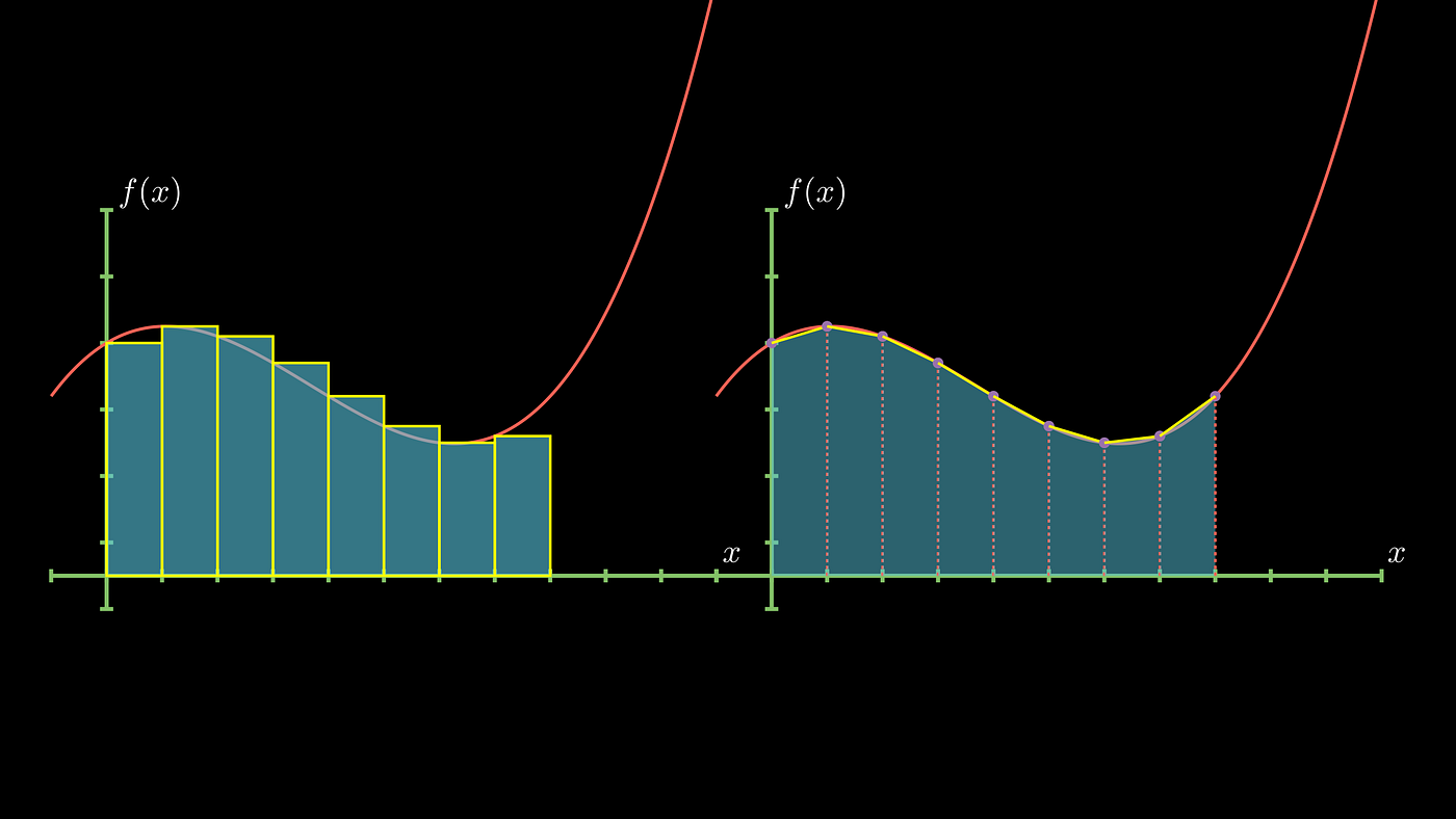
As you can see, I’ve used same number of rectangles and trapezoids in both cases with same width . Now it’s clear that trapezoids approximates the area better than rectangles which is the main idea behind using Trapezoids instead of Rectangles.

Calculating Area

Suppose we have a function f(x) and we are interested in the integration in the linear range of x = a and x = b. Then the value of integration is:

We have divide the x axis uniformly into small lengths ,each having a width of h = (b-a)/n . Here n(no. of trapezoid) is a huge number. The larger n will give us better result.

As the length is equally divided into n equal parts , hence we can write any point on x axis as

Corresponding to each of those x values , If we draw lines parallel to y axis , then the points at which they intersect the curve are the corresponding function values and hence the length of each dotted lines.

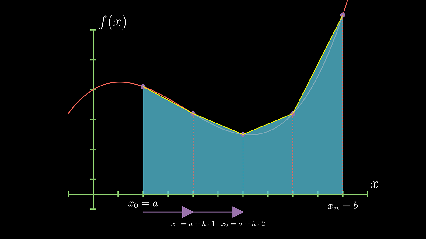
You may ask why x_r has such a value ? You can see in the figure-4, As we move from x_0=a to the end of the first trapezoid, we add it’s width to our x value. Hence, each time we cross a trapezoid , we have to add a h with the a. So, to reach the r-th point on x axis(r-th x value) we have to add h , r-times with our x_0.

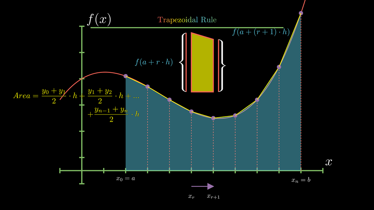
As you can see each shape is a trapezoid. Hence we just need to find the area of each trapezoid and adding them will give us total area under the curve.

Now you see we take two point x_r and x_(r+1). For those two points we have two lines parallel two y axis, whose lengths are f(x_r) and f(x_(r+1)) . You can see clearly it is indeed a trapezoid with a height of h(x_(r+1)-x_r) and the length of 2 parallel sides are the length of the lines which are parallel to y axis. Using just normal geometric area formula of trapezoid, we get,

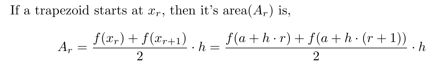
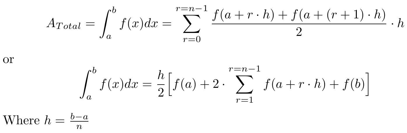
So , for a single trapezoid the area is as shown. Now for the total area we just sum over all. The index(r) will run from r = 0 to r = (n-1), where n is the no. of trapezoid or no. of division between x= a and x = b. Hence the total area of the region or the value of integration is (with a few error):

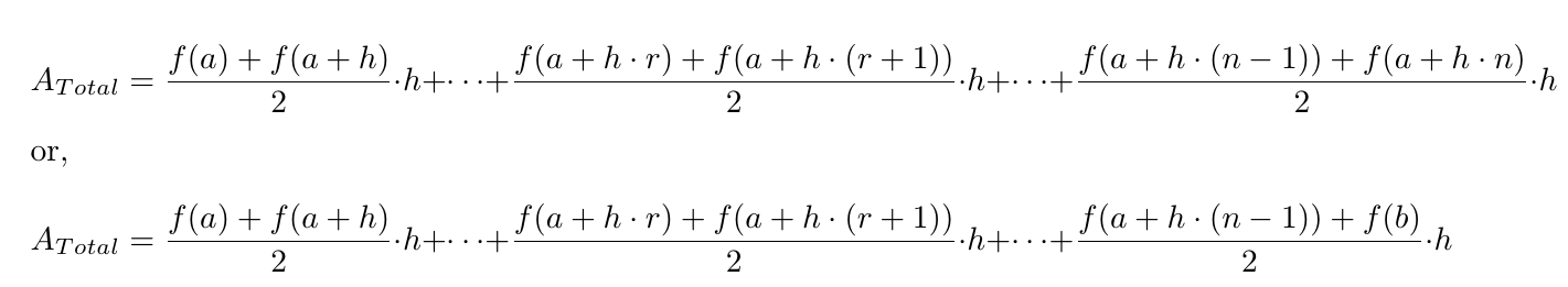
Using the summation notation, we obtain:

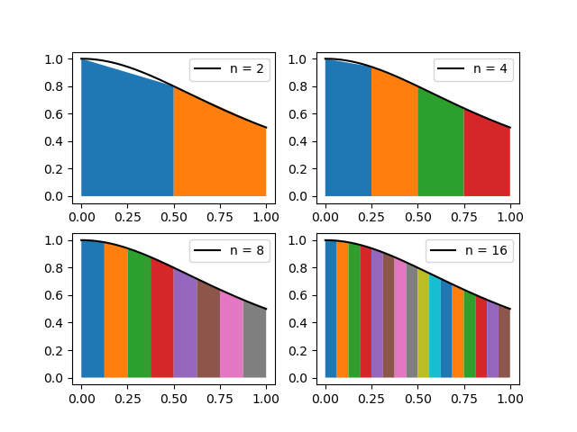
The upper formula works fine but for better approximation, we have to make n bigger, which makes h much smaller, giving us a result as perfect as we desire.

As you can see in the video above, as we decrease the value of h, i.e., increase the value of n, the area approximation(the value of integration) goes to it’s true value (i.e., reducing the value of error). Now, let’s see how you can use a computer to solve any integration numerically (we will use python):

Integration using Trapezoidal in Python

Algorithm

1. Define f(x), the function which we want to integrate.
2. Get the values of a , b, tolerance(The error value, i.e., |real value- calculated value|).
3. Assign the values of fa = f(a), fb = f(b), n .
4. Use a loop to perform summation.
5. Return or print the value.

Code

I have written it as a function so that we can use it at any time(it just uses numpy, although the program will work fine without it, just remove the pi value in the 2nd line with it’s true value):

This is a simple program. You can make it a little more user friendly by supplying the value of n, when calling the function.

Here is another(it just use numpy and matplotlib):

This code not only gives you the freedom to give any value of n but also shows how trapezoids cover the area under the curve. But as you can see i have removed the tolerance as it’s meaning-less when you are trying to learn how it converges. Although you can add it yourself like I did in the previous one.

You can see that there is some error in both cases(i have included the error in output). The amount of error in this method is proportional to the product of the second order derivative of our function f(x) and h².

If we include the error term, then the final expression will be,

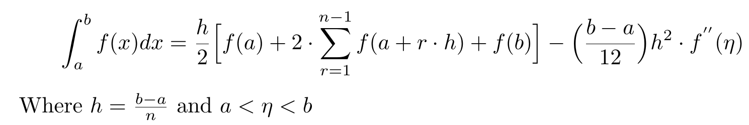
You can see clearly from the above expression that as we decrease h (i.e., increase n), the error term decreases.

Ending

As you can see, how beautifully we can use simple elementary geometry of trapezoids to approximate and compute integrations numerically. This is indeed powerful and much better than the classical rectangular approximation of area. Try It yourself, Solve some integration using this Trapezoidal Rule.

I hope you enjoyed learning something new.

Copyrights

All the programs, images and gif used here are all created by me using different python library and all equation are written using Tex. The pdf which is linked is taken from the book “What is Mathematics?” by Richard Courant and Herbert Robbins .