Your business involves repeatedly predicting the outcome of a gamble — the success of acquisitions, the return from investments, the repayment of loans — and you have subjective assessments of similar gambles that you or others have made in the past in the form of some sort of score.

This article describes a method for turning the straw of historical scoring into the gold of future probabilistic prediction.

How good are those assessments? Are they telling you anything? Do you have enough?

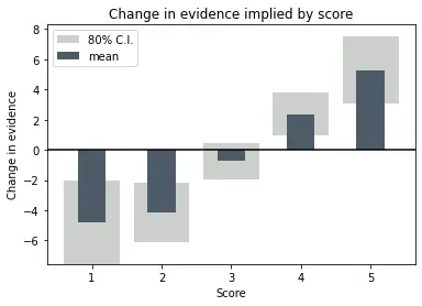
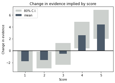
We’ll end up with a figure like the one above that shows exactly what a score is telling you about probability of success, with uncertainty bounds that show how well that message is supported by the number and consistency of the data.

This article (and all my mathematical articles) are aimed at readers with reasonable facility with high school mathematics. All the same, you ought to be able to skip the equations and still understand the gist of the article.

As an example, imagine a venture capital fund that invests in start-ups. Part of the investment approval process involves calculating a score on a scale from 1 to 5. The score may be for one particular aspect of the prospect or for the prospect as a whole; the method is the same. The fund has data on these appraisals going back several years. Do these scores tell the firm anything about future investments?

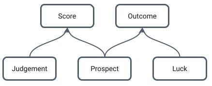
The success of the venture is a function of the quality of the prospect and a whole gamut of other factors over which we have no control, which we’ll just call luck. The score is (hopefully) also a function of the quality of the prospect and a whole gamut of other factors over which we have (maybe) a little control, but not a whole lot of knowledge. We’ll call these judgement.

The rigmaroles of regression

On the face of it, this looks like a regression problem. We just need to look historically at what success looks like as a function of score. Obviously Luck and Judgement will generate a lot of noise, but regression is exactly designed to tease relationships out of the noise.

The problem is clear if we redraw the causal map to show the relationship between variables in our database. Here, there’s one more arrow we need to draw: a big fat arrow from Judgement to Prospect, because we only have information for prospects in which we chose to invest.

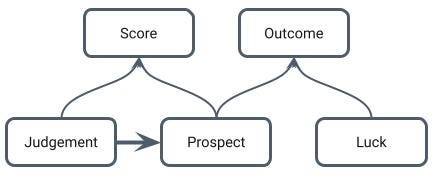
Now judgement is no longer noise we are trying to aggregate away, it has become a cumbersome confounder, reducing our regression to revealing the relationship between prospects we choose and their outcome, but we need to find the relationship between projects we consider and their outcome in order to know whether we should choose them.

Bayesics

The average success rate of the kind of start up that the fund supports is 20% (according to the fund’s criterion of achieving a certain return over a given timescale), so in the absence of any other information, the probability of success is 20%.

We can use Bayes theorem to modify this probability in the light of the information contained in the score. Say the prospect we’re looking at gets a score of 4. Bayes’ theorem in its basic form looks like this

The variable “outcome” can be success, denoted S, or failure. Here I’ve chosen success to see how the probability of success changes when the score is 4. The little vertical line on the left hand side is read as “given” so the probability here is the probability that the outcome is a success given that the score is 4.

The probability the outcome is a success on the right hand side is not given anything, so this is the probability before we’ve been given the information that the prospect has been given a score 4, i.e. 20%. So Bayes’ theorem is telling us how to update the probability of success with the information that the score is 4, which is exactly what we need.

The ingenuity of inversion

The first thing we need to make this calculation is the probability that the score is 4, given that the outcome is success. Presumably we have some successes in the database, so we ought to be able to infer the probability that successes are given a score of 4. Because outcome has a much weaker dependence on judgement than prospect selection, we can reasonably assume successes in our database are representative of successes in general, in a way we simply can not assume than prospects in our database are representative of prospects in general.

So far so good, but the other probability we need, the probability the score is 4 in general, i.e. not conditioned on success or failure, plunges us straight back into the regression rigmarole.

The beauty of evidence

The usual way to deal with this (expanding the probability the score is 4 using the law of total probability) makes an unholy mess of Bayes’ already slightly lopsided equation.

But, as I showed in my “Bayes Theorem Unbound” article, if we use Evidence instead of probability then Bayes’ theorem is transformed into an object of sublime elegance and power.

What is Evidence

Evidence is just another way of writing probability. For every probability between 0 and 1, there’s a value of evidence between negative and positive infinity. To go from probability to evidence, we use

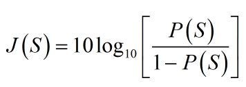
where J(S) is the evidence corresponding to the probability P(S). (J is for Jaynes) I’ve also gone over to the conventional, but potentially slightly confusing abbreviation of just writing S instead of “outcome = S”.

The relationship between probability and evidence is shown here. There’s also an equation that takes you back to probability from evidence.

Bayes unbound

Shifting back and forth between probability and evidence is frankly a bit of a pain, but it is a sacrifice amply compensated by the power and elegance of Bayes’ theorem when transformed to evidence

I’ve written D for datum, which in this case is a particular value of a score, but which can be anything — membership of a certain category (start ups whose founders are PhDs, start ups whose founders are Sagittarians) or a continuous variable (founder’s IQ, founder’s age in fortnights). The only requirement on D is that we can infer the probability of of seeing that datum in both the success and failure cases.

The equation tells us that the evidence for success, given the datum, is the evidence for success without the datum plus a number that we can reasonably infer from our database. This is illustrated below.

We start with a probability P(S), convert it to evidence (equation 2), then the amount of additional evidence contained in the datum D pushes us up or down the vertical axis, essentially sliding us back and forth along the evidence curve. We then convert the evidence we land on back into probability.

This form of Bayes separates the historical information about the datum from the particular instance we’re looking at. This means, we can look at things like scores and ask ourselves “Is this score telling us anything? Can it move a probability?”

But first we have to infer the missing probabilities.

Inferring probabilities from historical data

We go back to our example datum, that the score is 4. We need the probability that the score is 4 if the prospect is a success and if the prospect is a failure.

All the entries in our database of past prospects are either successes or failures. We can see the database as the results of two experiments, one looking at successes and one looking at failures.

Let’s say there are 80 successes and 77 failures. Broadly speaking, if the probability of a success being a 4 is 40% then we would expect roughly 40% of the 80 successes, i.e. 32, to have a score of 4.

We can turn this thought process around and argue that if 28 of the 80 successes have a score of 4 then 28/80 = 35% is probably not a bad guess at the probability that the score is 4 for success cases.

Example

Let’s say the number of successes with score 1, 2, 3, 4 and 5 are 2, 7, 25, 28 and 18 respectively. The numbers of failures are 9, 20, 29, 15 and 4.

Using this reasoning we infer the probabilities of getting a score of 1, 2, 3, 4 and 5 in the success case are 2/80 (3%), 7/80 (9%), 25/80 (31%), 28/80 (35%) and 18/80 (23%).

The probabilities of getting scores of 1, 2, 3, 4 and 5 in the failure case are 9/77 (12%), 20/77 (26%), 29/77 (38%), 15/77 (19%)and 4/77 (5%).

These probabilities are shown here. Visually, you can see that the distribution of scores is shifted to the right in the success case, so the score is telling us something.

The change in evidence implied by a score of four is

If we look at the evidence curve above we can see that 2.5 dB of evidence isn’t moving the probability enormously. Repeating the calculation, we get the following changes in evidence for each score

So 3 is neutral and 4 is mildly positive, but 5s do well and 1s and 2s do badly. At least on the face of it. The question is, how confident can we be that we have inferred those probabilities accurately?

To get the uncertainty range on this figure, we need a Bayesian approach, but as long as we’ve sold the frequentist farm and moved to the Bayesian uplands anyway, we may as well shop for some Bayesian inference here, too.

Inferring probabilities probabilistically

A Bayesian approach starts with a state of pure ignorance regarding the five probabilities corresponding to the probability of getting each of the five scores in, say, a success case. All we know to start with is that the five probabilities have to add up to 1, because every success case has one of the five scores.

The Bayesian approach takes each success case in the database as a datum that modifies this state of ignorance and generates a new description of how the probability is distributed between the five scores. We can turn this description into an uncertainty range on each of the probabilities.

This figure shows the starting point. Before we look at any data, each score has the same uncertainty (light grey) and is equally likely on average (20% — dark bars).

Now we take one of the success cases out of the database and look at its score. It’s a four.

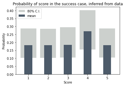
Now the probability that a success has a score 4 has gone up and the other probabilities have gone down. Not a lot, though. We have to keep going to really see the pattern emerge and the uncertainty ranges narrow.

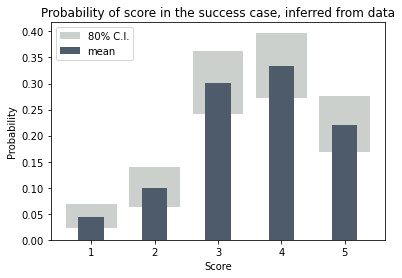
When we’re finished the probabilities look like this. The averages are close to, but not quite the same as the ones we calculated above and we now have an uncertainty range for each of the probabilities.

We do exactly the same for the failure cases and finally we calculate the change in evidence in equation 4.

Because we want to see how the uncertainties in the probabilities influence the uncertainties in the change of evidence, we have to do this probabilistically. We do this using a Monte Carlo simulation. A little quick one.

The final relationship between change of evidence and score, with the uncertainty range, looks like this.

We can see that the high scores are pretty solid in their prediction of improved probability, but there are indeed too few data to say with much certainty that a low score is a deal breaker.

Perspectives

This method, apart from giving a robust method for inferring a probability on the basis of a score, gives a wealth of information about the significance of different scores.

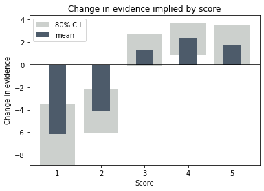
Scores that give figures like this are quite typical. Here a low score is clearly bad news, but a high score doesn’t tell you very much at all. Scores occasionally fall the other way too, where a good score is good news, but a poor score isn’t necessarily a coffin nail.

Of course scores with profiles like the following are all too common. Here there is enough of a sense of a trend that we can persuade ourselves they’re saying something, but in reality containing no useful information whatsoever. If this method does nothing else, rooting these out and showing them for what they are is enormous value in itself.