
The Worst Theoretical Prediction in the History of Physics
Dark Energy, and One of the Most Famous Unsolved Problem in Physics


Quantum field theory or QFT is the framework in which the Standard Model of particle physics (which includes the theories of the electroweak and strong nuclear interactions) is formulated. In particular, quantum electrodynamics or QED has predicted the values of physical quantities with unprecedented precision. For example, the magnetic dipole moment of the muon has a measured value of 233 184 600 (1680) × 10⁻¹¹. The theory predicts the following value 233 183 478 (308) × 10⁻¹¹. This agreement is nothing short of astounding (see this link).
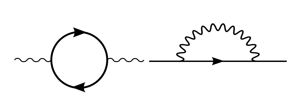
However, quantum field theory is also famous for its divergences. Perhaps, the most significant one regards the vacuum energy density (or vacuum expectation value, usually referred to as VEV), discussed in a previous article (see link below). Every quantum field has a corresponding divergent zero-point energy. Summing over all modes (until some physically reasonable energy or frequency cutoff) leads to a gigantic value for the vacuum energy density.
However, the vacuum energy predicted by general relativity and observed experimentally is extremely small. The difference in both estimates can be as high as 120 orders of magnitude (check this link).
The cosmological constant problem, also known as vacuum catastrophe, one of the most important unsolved problems in modern physics is precisely the existence of such discrepancy between the experimentally measured value of the vacuum energy density and the theoretical zero-point energy obtained using quantum field theory, which is much larger (see the link below). Hobson, Efstathiou & Lasenby (HEL) refer to it as “the worst theoretical prediction in the history of physics.”
When gravity is considered, such an energy density leads to severe difficulties since, in general relativity, any form of matter or energy must be added to the vacuum energy (in the case of the other fields, the vacuum energy can be subtracted, as will be discussed later).
The Energy of the VacuumQuantum Vacuum Fluctuations and the Casimir Effecttowardsdatascience.com
A Very Quick Overview of Einstein’s Gravity Theory
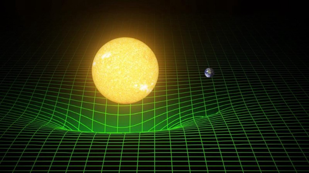
Between 1915 and 1916, Einstein concluded the formulation of his general theory of relativity. His gravity field equations showed that the warping of a spacetime region is generated by the nearby energy and momentum of the matter and radiation.
The following diagram illustrates the mutual correspondence:
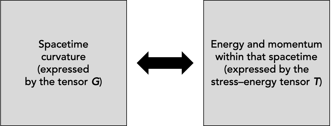
Written in terms of tensors G, R, and T the equation reads:

For a much more detailed treatment of the gravity field equations, check the following article:
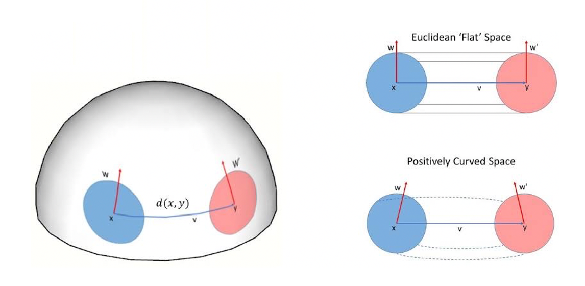
The tensor R, the Ricci curvature tensor measures the extent to which the geometrical properties of spacetime differ (locally) from that of the usual Euclidean space.
The tensor g in Eq. 1 is the metric tensor g, and has the form:

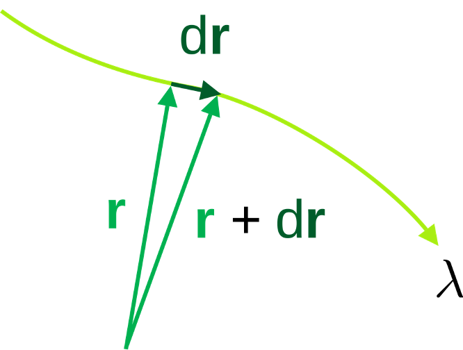
The corresponding line element (representing the infinitesimal displacement) can be written as follows:

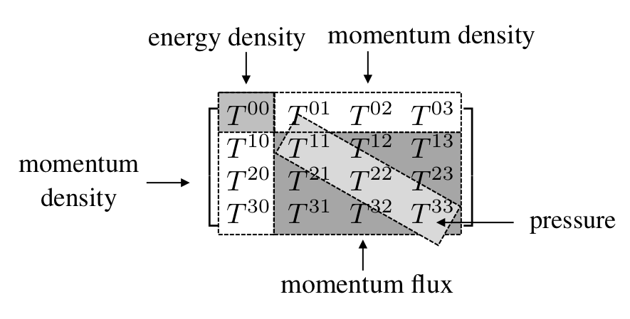
The tensor T on the right-hand side is the energy-momentum tensor. It contains information about the matter and energy which deforms spacetime.
A Bird’s-eye View of Cosmology
In 1917, one year after publishing his general theory of relativity, Einstein applied it to the entire universe (which was thought to be just only the Milky Way galaxy) in his seminal paper “Cosmological Considerations on the General Theory of Relativity.” This paper marked the birth of modern cosmology.
In this article, Einstein assumes the universe to be static and to have a closed spatial geometry (a three-dimensional sphere, which is finite yet unbounded). However, his theory did not admit static solutions (there were only contracting ones), and he had to introduce a new term (and an appropriate mix of matter and vacuum energy), the cosmological constant Λ term in Eq. 1:

This universe is known is the Einstein static universe and it is not of empirical interest (see Carroll).

He was able to include this term dependent on g in Eq. 1 for the following reason. The covariant derivative ∇ of both G and T is zero:

Since the metric tensor also has this property

the consistency of the equation is not spoiled by introducing the term. In the weak-field (or Newtonian) limit, we obtain:

We see that Λ acts as a gravitational repulsion, linearly dependent on the distance r.
The Expanding Universe
However, in 1929, the American astronomer Edwin Hubble found that:
- Several objects thought to be clouds of dust and gas were in fact galaxies beyond the Milky Way (this wasn’t known when Einstein introduced Λ into his equations).
- The recessional velocity of galaxies increases depending on their distance from the Earth (the so-called “Hubble’s law”)
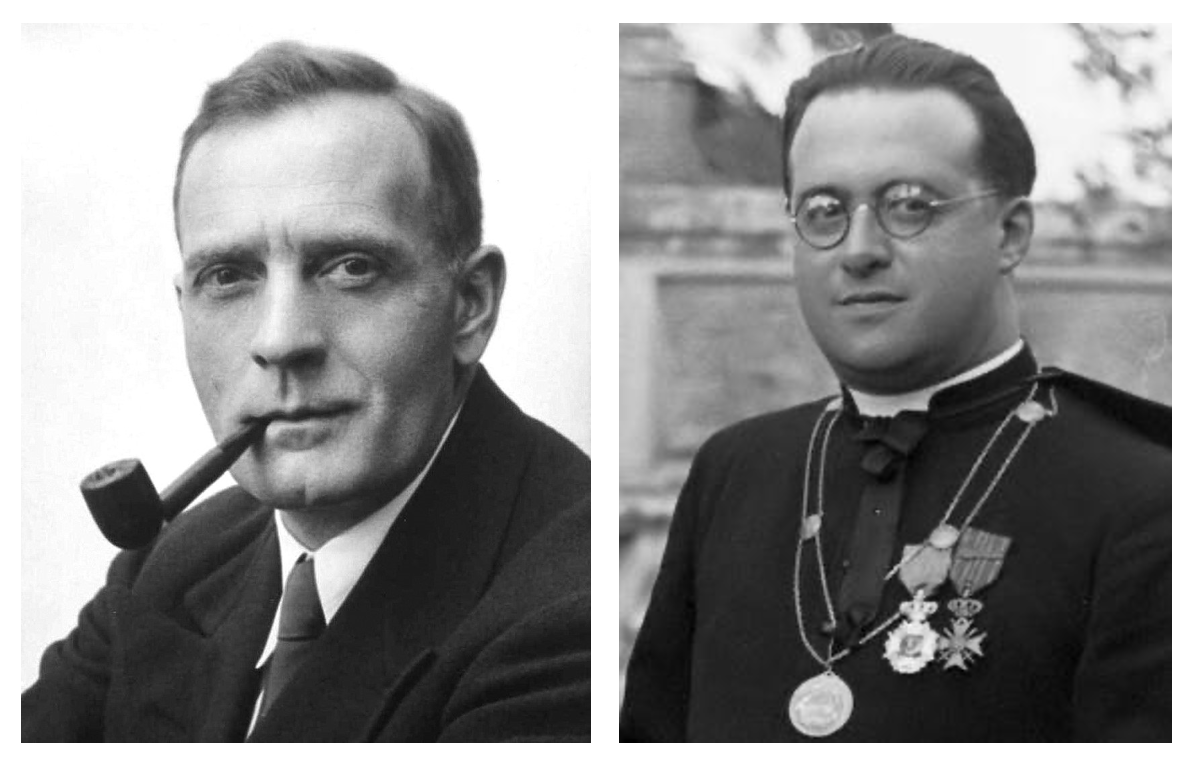
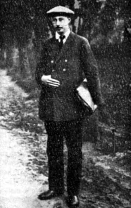
- His findings together with previous work by the Belgian Catholic priest, mathematician, and astronomer Georges Lemaître concluded that the universe is expanding.

The expansion of the universe meant, therefore, that introducing the cosmological constant wasn’t necessary, as Einstein thought. In a conversation with the Ukrainian born physicist and cosmologist George Gamow, he famously remarked that the introduction of the cosmological term was the biggest blunder he ever made in his life.
A Different View of the Cosmological Constant
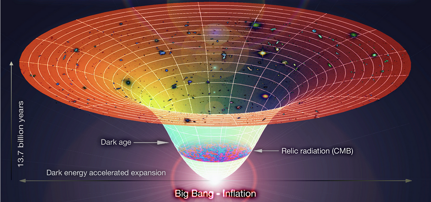
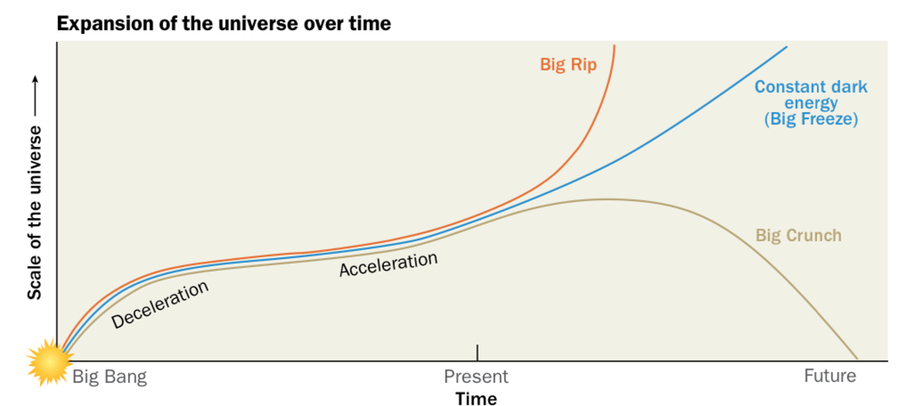
Today, however, the cosmological constant is viewed in a completely new way. In fact, its presence is responsible for the following spectacular experimental result: our universe is not just expanding, it is expanding at an accelerated rate. The phases of the expansion are illustrated in the figure below. Accelerating expansion occurs when the velocity at which distant galaxies are receding from observers is increasing with time.
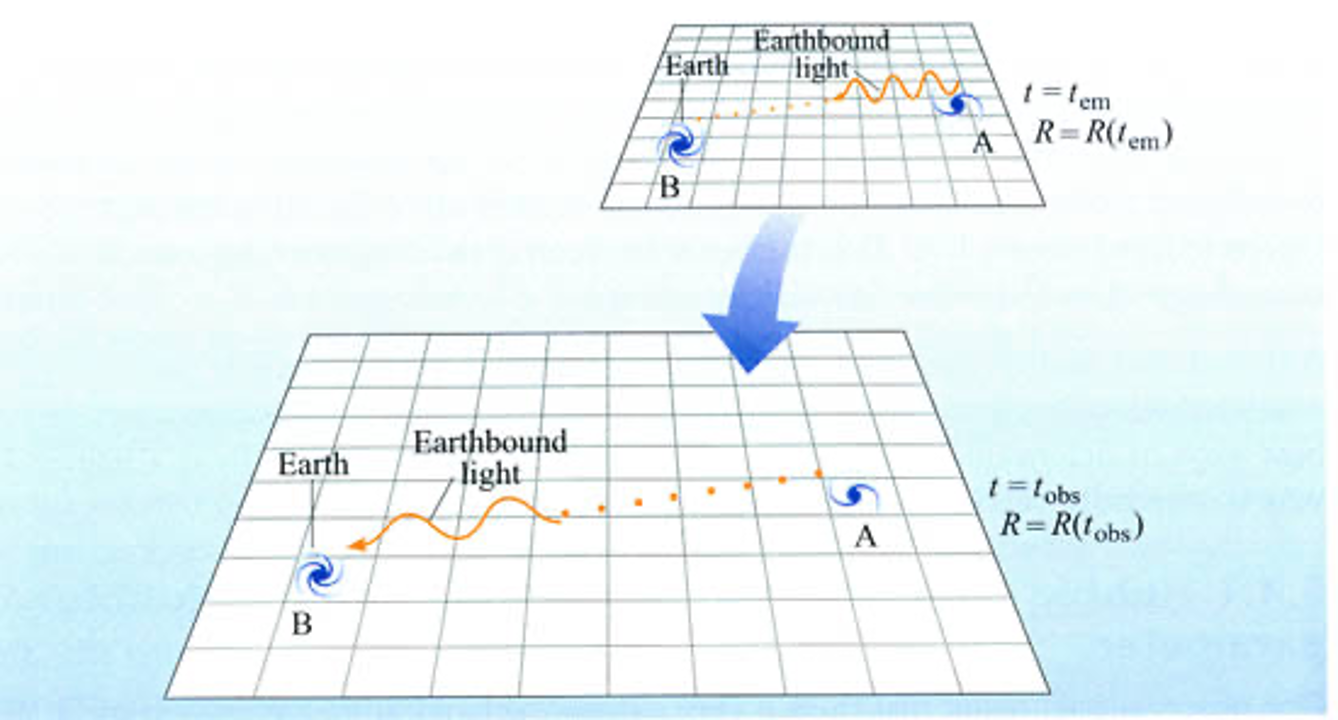
The Friedmann–Lemaître–Robertson–Walker (FLRW) Metric
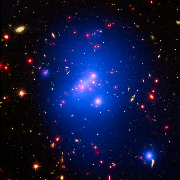
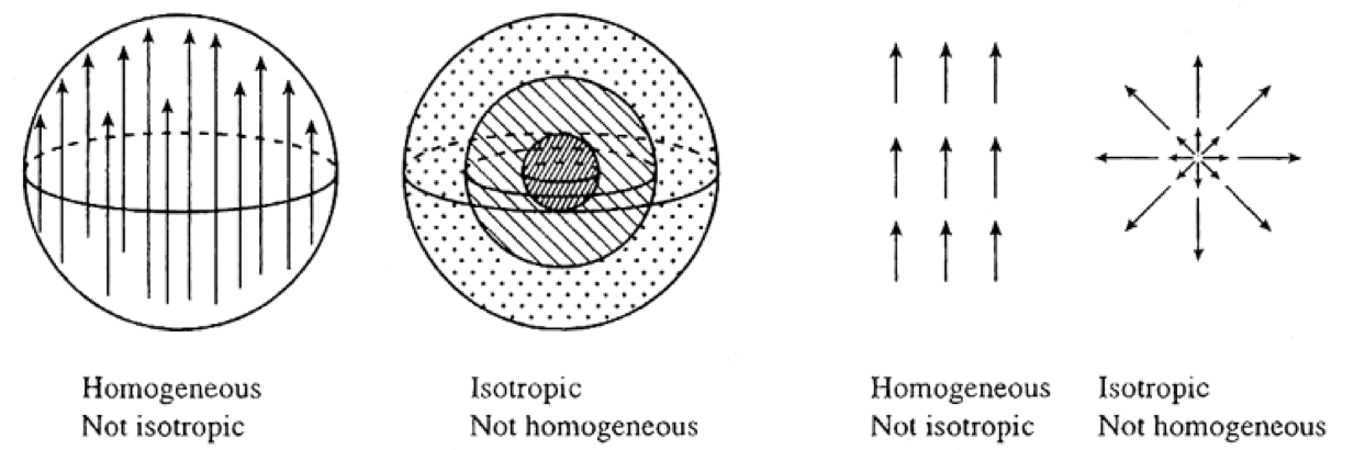
If one considers very large regions (such galaxy clusters, on scales of the order 100 Mpc where a parsec pc is equal to 31 trillion kilometers) the geometry of the universe (the spatial part of the metric), is approximately homogeneous (it is the same in all locations) and isotropic (it is the same in all directions). See Figure 10 below.
The figure below illustrates the concepts of isotropy and homogeneity:
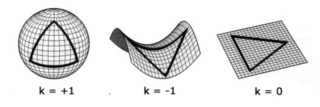
Based on these assumptions, one obtains as solutions of Einstein field equations, universes with constant curvature, the so-called Friedmann-Lemaître-Robertson-Walker (FLRW) universes. Their spatial part can be written in different ways.
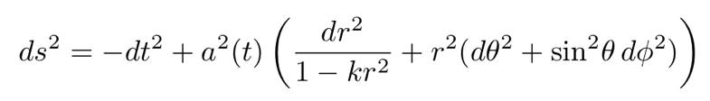
One possible choice is:

where the function a(t) is the cosmic scale factor, which is related to the size of the universe. The parameter k specifies the shape of the FLRW metric. The three possible values of k are +1,0 or 1 and are associated with universes with positive, zero, and negative curvatures, respectively.
Introducing spherical coordinates:


and defining the coordinate:

where the ~ identifies the usual radial variable the FLRW metric, and now including the temporal part the line element becomes:
It is important to understand that, points in spacetime and spacetime coordinates are two different concepts. Coordinates are labels assigned to thepoints and therefore their choice shouldn’t change the laws of physics. The coordinates r, θ, and ϕ are referred to as comoving coordinates. As the cosmic scale factor, a(t) increases, the distance between points also increases but the distance in the comoving coordinate system does not.
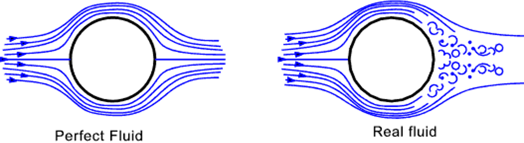
Assuming isotropy and homogeneity at large scales the energy-momentum tensor T becomes the energy-momentum tensor of a “perfect fluid”:

where ρ is the mass-energy density and p is the hydrostatic pressure.
A perfect fluid by definition:
- Is completely characterized by its rest frame mass density ρ and its isotropic pressure p.
- Have no shear stresses, viscosity, or heat conduction (see this link).
For example, consider T in its rest frame. It becomes simply:

With this simpler T we can describe matter using only two quantities: its density ρ and pressure p:

Note that both depend only on the cosmic scale factor a(t). The Einstein field equations then become the well-known Friedmann equations for the scale factor:

The third important equation is the equation of state which is just the equation on the right of Eq. 6 for FLRW universes:

Now consider, following HEL, some unknown substance with a particularly unusual equation of state, with negative pressure:

The tensor T, in this case, becomes (see the expression for T for the perfect fluid):

which is independent of the choice of coordinates. Note that T depends only on the geometry of spacetime (via g). It is, therefore, a property of the vacuum itself. Therefore ρ is the vacuum energy or energy density of space.
Now compare Eqs. 5 and 19. The new term has the same form as the g term. We can then write:

Therefore, the presence of the cosmological constant is equivalent to the existence of a vacuum energy density:

Einstein’s field equations then become:

Solving Eq. 16 for this case we obtain:

Cosmological observations give:

The Lambda-CDM model
According to the Lambda-CDM model, the accelerated expansion started after the universe entered its dark-energy-dominated era.
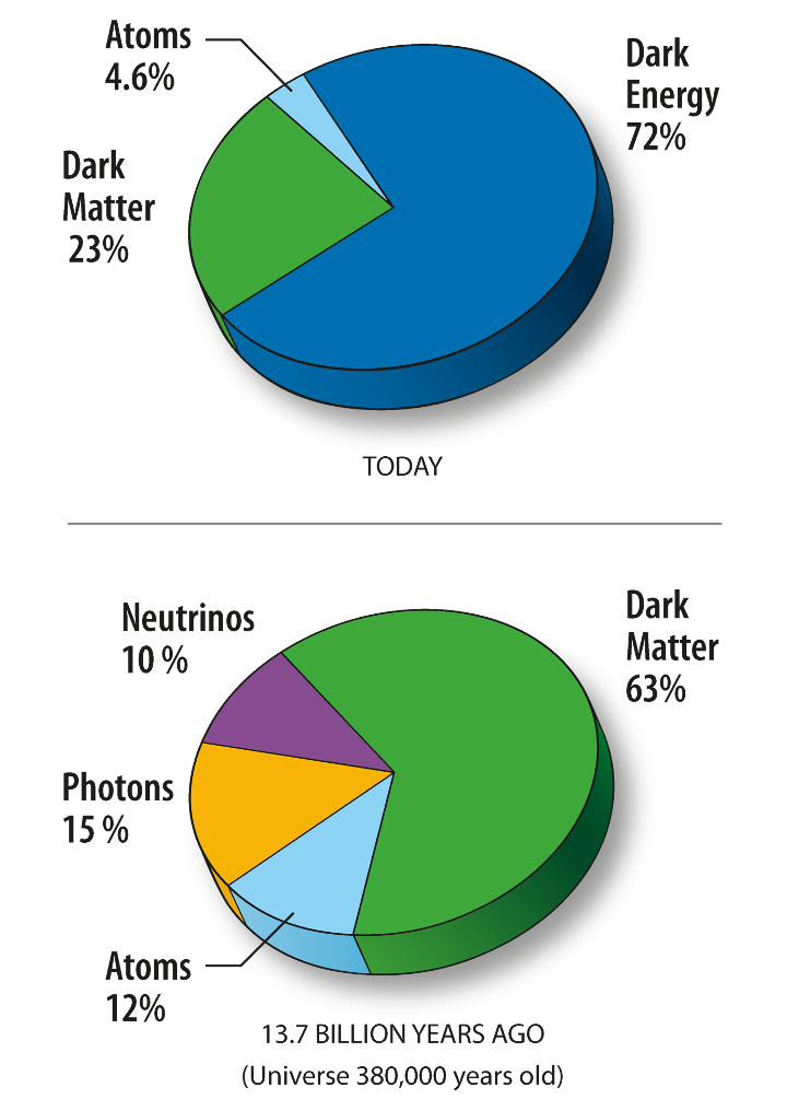
As explained before, the acceleration can be accounted for by the positivity of the cosmological constant (Λ>0). The latter is equivalent to the presence of a form of energy, dubbed dark energy, a positive form of vacuum energy. The description mostly used today in the current standard model of cosmology includes the presence of both dark energy and of the postulated dark matter.
However, as noted in Carroll (and mentioned in the introduction of this article), general relativity has the following peculiarity: while in non-gravitational physics (electromagnetism for example), only differences in energy are relevant to describe the motion of bodies (the zero of energy is arbitrary), in general relativity the value per se of the energy must be known. This leads us immediately to the question: if the zero of the energy is the energy of the empty state, what is the vacuum energy? One of the most important unsolved problems in physics is how can to answer that question.
Calculating the Vacuum Energy in Quantum Field Theory
Using quantum field theory one can calculate the quantum mechanical vacuum energy (or zero-point energy) for any quantum field. The result of this calculation can be as high as 120 orders of magnitude larger than the upper limits obtained via cosmological observations. It is believed that there exists some mechanism that makes Λ small but non-zero.
Let us calculate the so-called quantum energy of the vacuum which exists throughout the whole Universe.
To avoid unnecessary complications I will follow consider a real massless scalar field φ (instead of the more convoluted electromagnetic field) which is described by a real function φ(x,t). The classical Hamiltonian, in this case, is:

Now canonically quantizing the classical field φ. The vacuum energy is obtained by taking the expectation value with respect to the quantum vacuum state:

Expressing the field in terms of creation and annihilation operators and performing simple algebraic manipulations we arrive at the following expression for the vacuum expectation value (where there are no particles).

The second term in Eq. 26 implies that the vacuum expectation value (VEV) is infinite. This infinite contribution to the VEV is what shows up as the cosmological constant. As noted by Carroll, the infinite value is not a consequence of a possible infinitely big space: it is a consequence of the modes with high frequency over which we integrate. If we limit the integration using some cutoff we obtain:

If QFT is valid for energies as high as the Planck energy we obtain:

Dividing Eq. 28 by Eq. 23 we obtain the (in)famous factor of 120.
Thanks for reading and see you soon! As always, constructive criticism and feedback are always welcome!
My Linkedin, personal website www.marcotavora.me, and Github have some other interesting content about physics and other topics such as mathematics, machine learning, deep learning, finance, and much more! Check them out!


