The Wave Equation

This is the fourth entry in my series on partial differential equations. In the first three articles, we talked about the one-dimensional heat equation, where it comes from, and how to solve it in a few simple circumstances. Now we’ll cover the second of the three “basic” partial differential equations that are important for physics, the wave equation (the third is Laplace’s equation). As before, we’ll show how the equation arises and we’ll cover some interesting applications. Unlike last time, this article won’t be broken into three parts. You might want to read the first article in this series, which was about the heat equation, before this one, but the second and third are optional.

Waves

A wave is a physical process in which energy is transported through space by a propagating disturbance of a physical field from that field’s equilibrium state. The function ψ(x,y,z,t) describing the wave is therefore a description of that field’s state at each point in space and each moment of time.

In this animation, the function ψ(x,t) will give the displacement of the string from equilibrium at location x at time t. This is an example of wave motion described by the changing state of a scalar field. An important property of waves that propagate in matter (like a travelling disturbance on a string or a sound wave) cause energy to move without any net displacement of the medium carrying the wave. Wave motion can also occur in vector fields, such as in the case of electromagnetic waves where the disturbance will be propagated by the electric and magnetic fields.

This animation shows an electromagnetic wave traveling in the y direction. At every point in space (this animation only shows the wave on one line parallel to the y-axis) the wave is described by the electric field vector E and the magnetic induction field vector B, which are parallel to the z and x axes, respectively, and whose magnitudes oscillate with fixed amplitude and frequency.

So having described the phenomena that we’re looking at, now we’ll find an equation that models these phenomena.

Derivation

The wave equation is the equation of motion for a small disturbance propagating in a continuous medium like a string or a vibrating drumhead, so we will proceed by thinking about the forces that arise in a continuous medium when it is disturbed.

To keep things simple, I will derive the one-dimensional wave equation using the example of a small disturbance propagating in a string. Although the range of interesting phenomena that can be described by the wave equation is vast, showing that the wave equation holds for arbitrary phenomena of the sort described in the last second requires some advanced mathematical techniques and developing them here would be a distraction. You can check out this Wikiversity article if you’re curious about what that would entail.

Let us consider a very thin, tightly-stretched string that has mass density ρ kg/m. At equilibrium, the string coincides with the x-axis and when it is disturbed its displacement at each point x and time t is ψ(x,t), which is in the y-direction. We don’t write y(x,t) because the label y is reserved for independent position variables. The string is under constant tension T and this tension will give rise to a restoring force that will attempt to pull the string back to equilibrium. For now, let’s assume that the tension force is strong enough that any external forces like gravity and air resistance are negligible by comparison. Then each particle of the string is therefore subject to the following equation of motion:

To complete the derivation we need to find a formula for the restoring force in terms of ψ.

Let’s consider a very short segment of string. For the graph of a continuous function, we can always find a sufficiently small Δx such that the the function is monotonically increasing or decreasing on the interval [x, x+Δx], without loss of generality we will consider an interval where ψ is increasing. Furthermore, for a small enough segment of string, it’s accurate to approximate the tension force as acting only at the ends.

The tension force is always tangent to the string and therefore to the graph of ψ for each moment of time. We’ve assumed that ψ is increasing so at x the tension force is directed down and to the left and at x+Δx to the tension force is directed up and to the right. Suppose that the tension force vector is at an angle θ₁ below the horizontal at x and at angle θ₂ above the horizontal at x+Δx. This means that the total vertical component of the tension force on the string is T∙[sin(θ₂)-sin(θ₁)] and the total horizontal component is T∙[cos(θ₂)-cos(θ₁)].

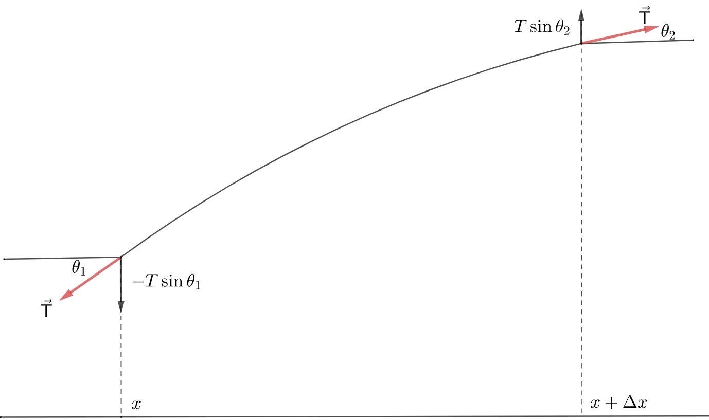
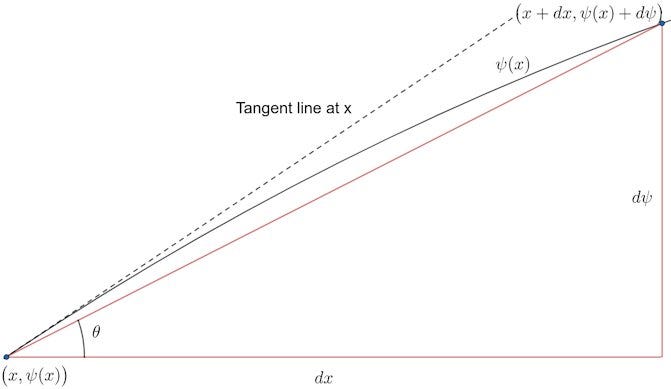
Since we’ve assumed that the displacement of the string is very small, we can use the small angle approximation. The result of this will be cos(θ₁)≈cos(θ₂)≈1 so the cosines of the angles are approximately equal and the horizontal component of the tension force on the segment vanishes. Furthermore, for small angles, sin(θ)≈θ≈tan(θ) and remember that for a right triangle the tangent of the angle is equal to the height of the triangle divided by the length of the base. At every point on the graph of a continuous function ψ we can construct an infinitesimally small right triangle whose base will have length dx, whose height is dψ, and whose hypotenuse is the line from (x,ψ(x)) to (x+dx,ψ(x+dx))=(x+dx,ψ+dψ). If the graph is approximately linear in this small interval then this hypotenuse is very close to the tangent line to the graph, so if θ is the angle between the tangent line and the graph then tan(θ)≈dψ/dx.

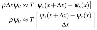
This means that sin(θ₂)-sin(θ₁)≈tan(θ₂)-tan(θ₁)≈ψₓ(x+Δx, t)-ψₓ(x,t), where the subscript x means partial derivative with respect to x. The length of the segment is Δx so its mass is ρΔx and this gives us enough to set up the Newton’s Second Law equation for the segment:

All of the approximations that we’ve used tend towards equality in the limit as Δx→0, and this will give us the wave equation:

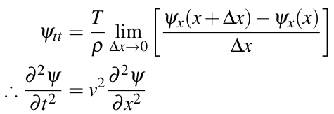
We made the assignment T/ρ=v² because T has units of kg∙m/s² and ρ has units of kg/m, so T/ρ has units of m²/s².

The extension to three dimensions is straightforward:

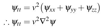
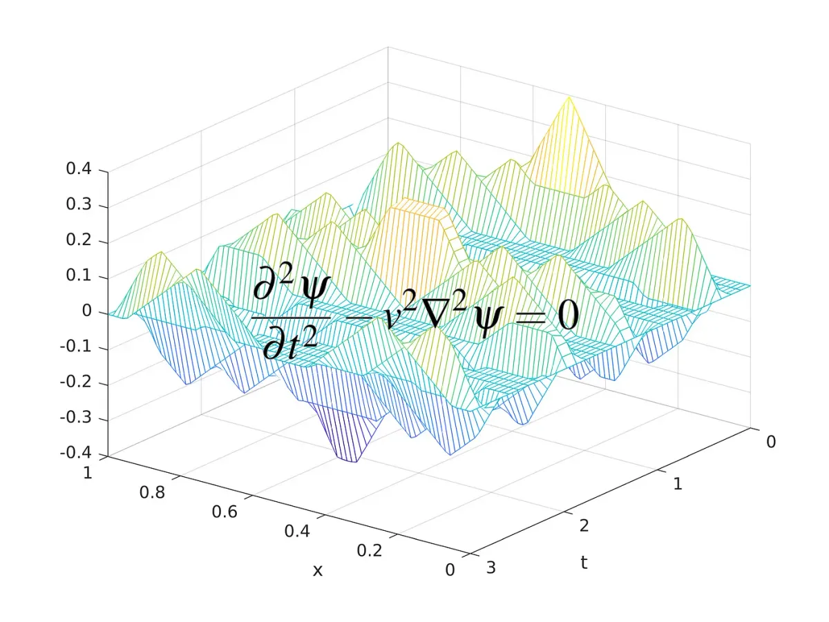
The wave equation is so important in physics that the operator ∂²/∂t²-v²∇² has its own name and symbol. We call it the d’Alembertian and it is defined by:

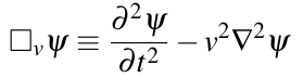
For waves that travel at light speed the subscript v is dropped and the wave equation is written as ☐ψ=0.

Solution: Separation of variables

When we talked about the heat equation, we found the solution by guessing and checking. This was possible because phenomena described by the heat equation are in a sense “simpler” than what can be described by the wave equation and this made it easier to use the expected qualitative behavior of the solutions to guess the form of the solution. We don’t have this luxury for the wave equation, so we will need to find the general solution directly. For this, we will use the method of separation of variables.

In separation of variables, we suppose that the solution to the partial differential equation can be written as a product of single-variable functions and then we try to use the partial differential equation to set up ordinary differential equations for each function. So let’s begin by assuming that ψ(x,y,z,t)=X(x)Y(y)Z(z)T(t), and then plug this into the wave equation:

Then divide through by v²TXYZ:

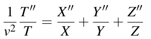
This must be true for all (x,y,z,t), for example if t, y, and z are held constant but x is changed, this equality must still be true. Therefore each term must be equal to a constant.

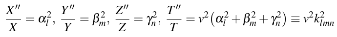
The constants are indexed because we expect that the general solution should be a linear combination of functions that each satisfy the equation and boundary conditions. These functions are called modes and each triplet (l,m,n) corresponds to a different mode.

These are elementary differential equations and their solutions all have the form Z(z) = Eₙcos(γₙz)+Fₙsin(γₙz). Then we obtain the general solution:

Now that we’ve developed the technique that we’ll be using, let’s look at some examples.

A triangle wave

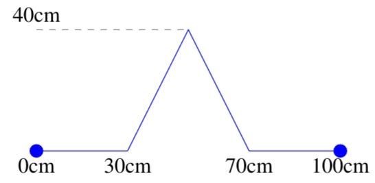
We’ll see how a wave travels back and forth on a string that’s clamped at the ends. The clamping at the ends means that we have the boundary condition ψ(0,t)=ψ(L,t)=0, and we’ll assume that the string is one meter long. The initial condition will be a triangular pulse with height 40cm and with a base that extends from x=30cm to x=70cm and we will assume that the string is released from rest in this condition at t=0 so that ψₜ(x,0)=0.

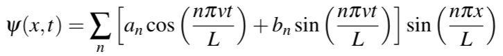
Since physical quantities like length are always real-valued, the solution that we’re looking for is the real part of the general solution to the one-dimensional wave equation:

The easiest way to satisfy the boundary conditions will be to set Aₙ=0, Bₙ=1, and relabel Cₙ and Dₙ as aₙ and bₙ, respectively. We have replaced kₙ with αₙ because they are equal in the one-dimensional case. Then αₙ=nπ/L will cause sin(αₙx) to be 0 for x=0 and x=L, so the general solution is:

Now we can find the Fourier coefficients aₙ and bₙ by taking inner products and using the orthogonality of the cosine and sine functions that we discussed in the heat equation article. We will generalize the initial condition slightly by assuming that it has height h, width 2w, and is centered at L/2, then it has the piecewise form:

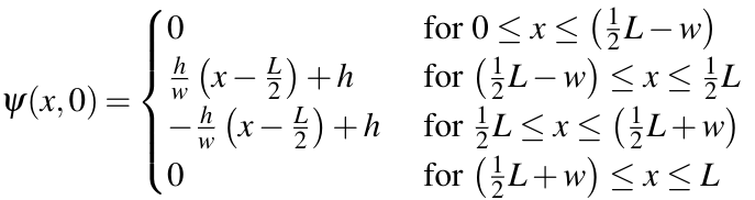
Then ψ(x,0) is also given by:

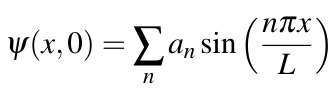
Then we get a formula for the Fourier coefficients by equating these two expressions for ψ(x,0) and taking the inner product of each side:

An expression like this is unlikely to result in Fourier coefficients that can be written down in a neat form so it’s best to evaluate them numerically. I’ll provide MATLAB code to do this.

Now we find bₙ by using the initial condition ψₜ(x,0)=0:

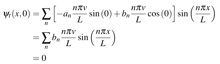
This means that bₙ=0 for all n. This means we have enough information to solve the problem. The solution is animated below.

Forcing

The one-dimensional forced wave equation is:

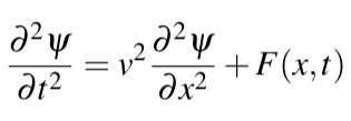
If the system that we’re modeling is a vibrating string, then the function F(x,t), called the forcing term, represents an acceleration at each point on the string in addition to the acceleration due to the restoring force.

As a simple example, let’s see what happens when we apply uniform gravity to the problem that we just solved in the previous example. The ends of the string are still clamped, so the forcing term is:

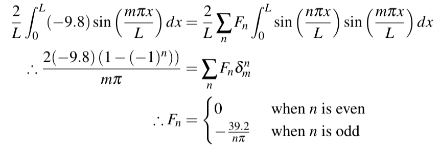
The approach here will be similar to what we did when we dealt with the forced heat equation. Recall that any function F(x,t) that’s piecewise continuous on 0≤x≤L and that satisfies F(0,t)=F(L,t)=0 can be represented as a Fourier sine series:

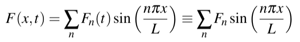
The coefficients Fₙ are constant if F does not depend on time. By now, finding these coefficients should be second nature to you:

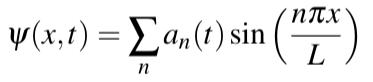
The general solution to this equation takes the following form:

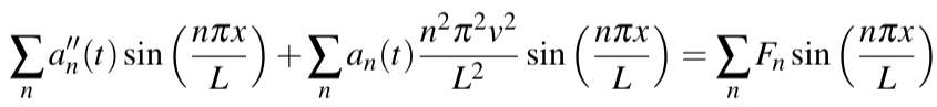
When we plug this into the forced wave equation, we get:

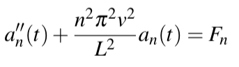
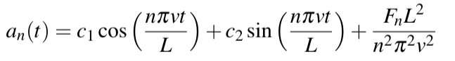
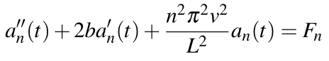
So for each n, we have an ordinary differential equation for aₙ(t):

The initial conditions aₙ(0) and aₙ′(0) are the Fourier coefficients for ψ(x,0) and ψₜ(x,0) from the unforced version of the problem, so aₙ(0)=aₙ and aₙ′(0)=0. The general solution to this ODE is:

Now we find the particular solution by plugging in the ICs:

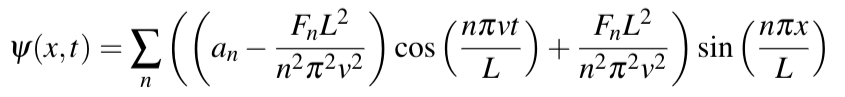
And this gives us enough information to write out the solution to the initial boundary value problem for the vibrating string acted on by gravity:

You can see the animation of the solution below:

Damping

Now let’s consider what happens when the string is subject to air resistance. From basic mechanics, we know that if a particle is moving with velocity v through a viscous medium, then there will be a drag force given by f=-kv where k is a constant that depends on the system. Since the velocity of the string is ψₜ, we can include the acceleration due to drag in our equation:

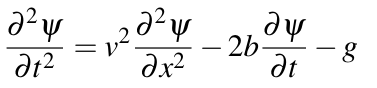
We use 2b instead of just b for the coefficient to make some calculations more convenient. We call 2bψₜ the damping term.

Damping causes an oscillating system to lose energy over time. The systems that we’ve looked at so far have been undamped, meaning that they stay in motion indefinitely. On the other hand, a damped system will eventually come to rest. Usually, b is a positive number. If b is negative, then the system is subject to “negative damping”, meaning that it accelerates in the direction of its velocity proportionally to the magnitude of the velocity, causing its kinetic energy to increase exponentially with time and in short order causing the system to blow up (possibly literally).

Once again, we’ll find a differential equation for aₙ(t) by plugging the general form of the solution into the damped and forced wave equation:

Then we obtain the following ODE for aₙ(t) for each n:

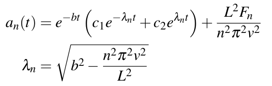
Remember that Fₙ are just the Fourier coefficients for uniform gravity. The general solution is:

Now we plug in the initial conditions, which again are just the initial conditions for the undamped and unforced problem, aₙ(0)=aₙ and aₙ′(0)=0. We then find the following system of equations:

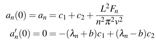
And this can be solved to give us the coefficients:

So the solution for aₙ(t) is:

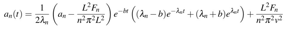
And the particular solution is:

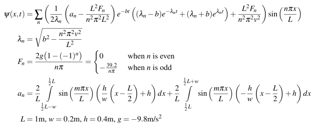
Here is the animation of the solution:

You can get the MATLAB code that I used here on Pastebin. We used v=0.5m/s for the first example and v=1.25m/s for the second and third examples.

Concluding remarks

This article may have seemed more mathematically involved than much of my other work, but ultimately the only real difficulty is getting through the grunt work without making any mistakes. The hard part is deriving your differential equation, but once you’ve done that then the recipe for solving the problem is simple: find the general solution by separation of variables and then find the Fourier coefficients that make the general solution match with the initial and boundary conditions. As I mentioned before, the range of phenomena that obey the wave equation is vast, and so much larger than what can be done with the heat equation. If you want to learn more, then truly the best way to is to think up some wave-like processes on your own and try to solve the equation for them.

Copyright

The images, animations, and code in this article are my own original work unless stated otherwise. I don’t care if you want to use them elsewhere as long as you attribute me. The MATLAB code that I linked should run without issue on any reasonably modern machine but obviously I cannot promise that it will work flawlessly for everyone.