In mathematics, there are thousands of theorems to be proven. Often, we tailor unique proofs for one of these theorems — this can be beautiful, but extremely difficult at the same time. Think about proofs to theorems that involve constructing a desired object.

As a small example, consider the following “theorem”:

You can prove this by constructing the desired x using one of several formulas or techniques:

We omitted the work needed to get to this exact number, but you know that there definitely is a bit of work, especially if you don’t know the solution formulas and how to derive them.

Another approach is proving the existence of a positive root in a non-constructive manner:

f is continuous. Note that f(0)=-1<0 and f(1)=1>0. According to the intermediate value theorem, there must be a c∈(0, 1), i.e. a positive c with f(c)=0.

Done.

The non-constructive proof is very short and easy to understand which makes it attractive. On the other hand, it is frustrating that we won’t know the object explicitly, although we want to. Also, constructivists would disregard this proof because they assert that it is necessary to find a mathematical object to prove that it exists.

Still, non-constructive proofs are a great and quick way to get things done. And no one prevents the constructivists from constructing the object afterwards. 😉

Now, let us get to an exciting framework for doing non-constructive proofs — the probabilistic method.

The Probabilistic Method

The idea of the probabilistic method, pioneered by Paul Erdős, is stunningly simple:

If an object exists with positive probability, it exists.

Well, duh! It sounds trivial, but this observation lets us prove the existence of many interesting things. But wait — why and which probability? It’s best illustrated with an example.

Edge Coloring of Graphs

Let us first define a few things. Let Kₙ be the complete Graph, i.e. an undirected graph with n nodes (circles) and all possible edges (lines) between all nodes.

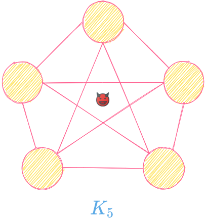
We can now take a brush and color the edges of graphs like these with exactly two colors. A theorem about the coloring of complete graphs goes as follows:

If we have

then it is possible to color the edges of the Kₙ with two colors so that it does not contain any monochromatic Kₖ subgraph.

Subgraph: You can obtain a subgraph of a graph by just deleting nodes and the corresponding edges.

Not containing a monochromatic subgraph: A graph with colored edges does not contain a subgraph having all the same colors.

If we plug in the values n=5 and k=4, the conditions for the theorem to be applied are fulfilled, as the left side of the inequality is 5/32. Therefore, it should be possible to color the ten edges of the K₅ such that it does not contain a monochromatic K₄. We just don’t know how so far. But by just trying around, we can easily find this one:

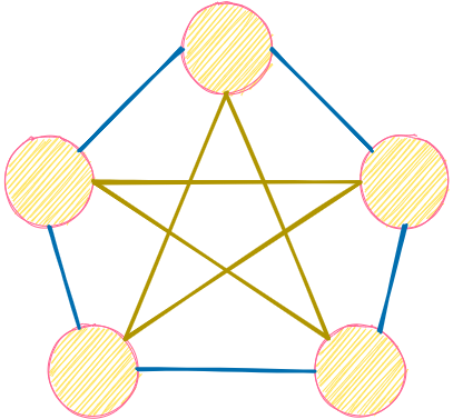
If you take any four nodes from the K₅ now, you can see that each subgraph that consists of these four nodes has edges of both colors.

Note: Using the same coloring as above, we can also see that the statement also holds for n=5 and k=3, although it is not covered by the theorem. Just try it out mentally, or draw it.

So, how can you prove such a theorem? Finding an algorithm to construct an edge coloring with the desired property seems intimidating. But fear not! The proof with the probabilistic method is easy.

Proof: Consider the Kₙ and color each of its (n choose 2) edges randomly with the two colors. What is the probability that some arbitrary Kₖ subgraph is monochromatic? Well, all of its (k choose 2) need to have the same color, which happens with a probability of

Alright, how many Kₖ subgraphs are there inside of the Kₙ? The answer is simply (n choose k). Let’s number them Kₖ¹, Kₖ², Kₖ³, …

Then, according to the union bound, we have

We know the last term from the theorem statement. It is strictly smaller than 1 by definition, which in turn implies for the counter probability

Thus, the probability that a random coloring induces only bichromatic complete subgraphs is larger than zero, so there must be at least one coloring with this property.

Otherwise, if there is no such coloring, the probability would be zero. ∎

Beautiful, isn’t it? By introducing a simple distribution over the colors of the edges, we could prove something deterministic.

There are even more ways to utilize the probabilistic method, for example using the expectation. Let us work through one example where we will prove an inequality that — again — does not contain any probabilities.

The Crossing Number of Graphs

Let’s start with a small definition.

The crossing number cr(G) of a graph G is the lowest number of edge crossings of a plane drawing of G.

Consider the K₄ as an example:

In this drawing, there is one edge crossing right in the middle, which implies that cr(K₄)≤1. Why “≤”? Because there might be a better way to draw this graph. For example like this:

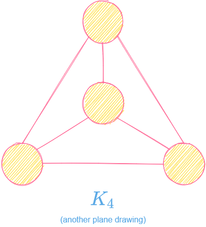
It’s the same graph, just with the nodes moved around in the plane. In this view, there are no edge crossings, hence cr(K₄)=0. We also call such a graph planar.

We have the following theorem:

Let e be the number of edges and n be the number of nodes of some graph G with e>4n. Then

This is an impossibility statement: It does not matter how smart we rearrange the nodes in the plane, there is always a minimum number of crossings that we cannot undercut. We can prove this again using the probabilistic method.

Proof (paraphrasing the proof on Wikipedia): First, one can show that cr(G)>e-3n using Euler’s formula. This is the non-probabilistic part of the proof.

Now, select a random subgraph H of G the following way:

• Choose some probability p.
• For each node in G, flip an independent 0–1 coin that shows 1 with probability p. In this case, choose the node for H. If the coin shows 0, the node does not belong to H.
• For each edge in G, put it into H if both end nodes of the edge are in H as well.

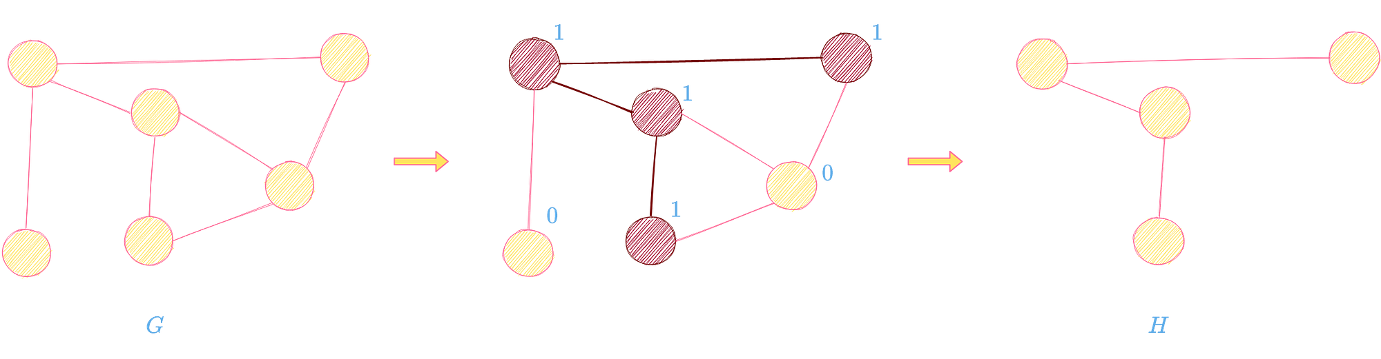
We will choose the value for p later. Let nₕ and eₕ and be the number of nodes and edges of H. Using Euler’s formula again, we receive cr(H)>eₕ-3nₕ. Since H is a random object, cr(H), eₕ and nₕ are random variables as well. So, let’s compute their expectations!

1. E(nₕ)=pn since each of the n nodes of G belongs to H with probability p.
2. E(eₕ)=p²e since each of the e edges of G belongs to H whenever both end nodes of e belong to H. This happens with probability p².
3. E(cr(H))=p⁴cr(G) since each of the cr(G) crossings of G belongs to Hwhenever all 4 endpoints of the crossing edges belong to H. This happens with probability p⁴.

Thus, applying the expectation to the inequality cr(H)>eₕ-3nₕ we receive

which is what we wanted to show. Note that 0<p<1 since e>4n, hence p is a proper probability. ∎

Conclusion

In this article, I introduced to you the probabilistic method for proving theorems. When using this method, you artificially introduce randomness to reach your goal, even if the theorem that you want to prove does not involve any probabilities. This makes it an extremely fancy and exciting way of proving things, in my opinion.

We have seen the probabilistic method in action when proving two different theorems about graphs. Further examples of non-probabilistic theorems that can be proven with the probabilistic method can be found on the Wikipedia page “List of probabilistic proofs of non-probabilistic theorems”. Among them are theorems from analysis, algebra, topology, geometry, number theory, quantum theory, information theory, and as we have seen combinatorics.

In some cases, this proof method can even be used to find the desired object of interest algorithmically. Take the first theorem from this article as an example: We can randomly color the edges and check if the Kₙ does not contain any monochromatic Kₖ. If the check is positive, we have our solution. Otherwise, randomly color the edges again, until this check is positive at some point. Since we find a suitable object with some probability p>0 (that is what we showed), we need to run this experiment expected 1/p times until we have a solution.

Whenever you sit in front of a problem now, the probabilistic method is a new tool that you could try out, besides induction, proof by contraposition, or contradiction. May it be helpful to you!

I hope that you learned something new, interesting, and useful today. Thanks for reading!