Binary search is ubiquitous. Even if you are not aware of it, you have most likely used some (approximate) version of binary search one way or another, for example when looking up a name in a phone book or a word in a dictionary (back in the day), or in any application where you are looking for an element among objects that have some kind of total order.

Binary search addresses and resolves the following problem.

Given a sorted list of items L and a target item t, check whether t appears in L, and if so, find the position in which it appears.

In this article, we will describe an optimal (worst-case) algorithm to solve this problem, where the cost of an algorithm will be the number of comparisons it makes in the worst case (this will be made more precise in the next few lines). Although many different kinds of items have a natural order, we will focus on the natural numbers. More precisely, we assume that we are given a list of n natural numbers, sorted in non-decreasing order, and a target number t, and the goal is to check whether t appears in L, and if it does, report its position. To simplify the analysis, we will consider one basic operation, which we call a “comparison” or “query”, and is the main unit of cost we will use. We define a comparison/query to be the following operation.

Given two natural numbers a and b, check whether

a < b, or a = b, or a > b.

From now on, our goal is to minimize the number of comparisons made by our algorithms in the worst case. At the end of this article, we will briefly discuss whether such a simplification makes the analysis loose or not.

Warm-up

Suppose we are given the following sorted list of 10 numbers

L = (1, 3, 3, 11, 18, 25, 45, 57, 57, 63),

and the target t = 57.

We observe that 57 appears in L, and in particular, it appears in two positions, the 8th and 9th position.

If we change the target number and ask for t = 15, then we observe that 15 does not appear in L, and so the answer to the problem should be “NO”.

The goal now is to design an efficient algorithm that solves this problem, for any sorted list L and target element t.

Note: from now on, we will denote the size |L| of the list as n.

An obvious solution: Linear Search

The first algorithm, which we call Linear Search, that comes to mind is to simply scan the list, from left to right, until we either find the number t, or reach the right end of the list, in which case the number t is not in L. In pseudocode, this simple algorithm looks as follows.

for i = 1,...,n:
if (L[i] == t)
return i;return "NO";

The above algorithm scans the list and reports the first position that the element t appears in, or it reports “NO” if the element t is not in L.

It is not hard to see that in the worst case, the algorithm goes over the whole list, does not find the element, and returns “NO” at the very end. Thus, the number of comparisons it makes in the worst case is n. We conclude that the the algorithm always makes O(n) comparisons, which, in the worst case, is tight.

Can we do any better?

If we look a bit more carefully at the above algorithm, we observe that it does not exploit in any way the fact that the list is ordered. In other words, the algorithm works even if the list is unordered. So, one might wonder whether we can exploit this (crucial) fact in order to speed up the algorithm. We will see that, in fact, we can have an exponential improvement in the running time, by exploiting the order in the list.

We start with a general observation. Any (deterministic) algorithm has to make a first query. Since we do not have any extra information about the way the input elements are distributed, the only information that we can extract from a query at position j, for 1 ≤ j ≤ n, is the following:

(1) whether the element t located at position j, or

(2) whether the element t is strictly smaller than the element at position j, in which case, if t appears in the list, it must be in some position with index from 1to j-1, or

(3) whether the element t is larger than the element at position j, in which case, if t appears in the list, it must be in some position with index from j+1 to n.

If we are in case (1), then we are done. On the other hand, if we end up in cases (2) or (3), then we observe that the remaining task is identical to the original task, except for the fact that the input size has reduced. In other words, any deterministic algorithm that only makes decisions based on the input size will necessarily have a recursive structure. Let T(n) be the number of comparisons between elements of the given list that such an algorithm makes when the input list consists of n numbers. Then, if on input size n it decides to first query position j (for some j that satisfies 1 ≤ j ≤ n), then its running time will be

T(n) = 1 + max{T(j-1), T(n-j)}.

In order to ensure that the above recursive equation is always properly defined, we also define T(0) = 0, which is trivially true.

Clearly, any “reasonable” algorithm satisfies T(n) ≤ T(m), for n ≤ m. To see this, note that if such a property is not satisfied for some input sizes n and m, with n < m, then we can always start by adding some padding in the beginning or the end of our list so as to make our list have size m, and then run the algorithm on this new list. Thus, from now on we assume that such a property is satisfied. This implies the following:

• if j-1 ≤ n-j, then we get T(n) = 1 + T(n-j). Equivalently, if j ≤ (n+1)/2, then T(n) = 1 + T(n-j).
• if j-1 > n-j, then we get T(n) = 1 + T(j-1). Equivalently, if j > (n+1)/2, then T(n) = 1 + T(j-1).

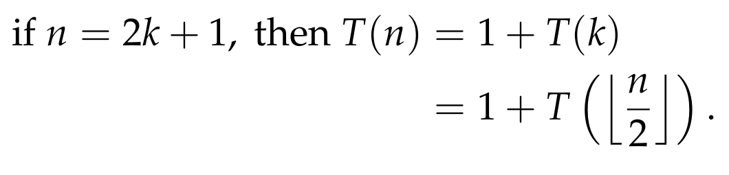
To get some intuition about the above, let’s assume that n = 2k+1, for some natural number k ≥ 2. In other words, let’s assume that n is an odd number that is at least 5. We do a case analysis based on what position j we decide to first query:

• j = 1. We have T(n) = 1 + T(n-1) = 1 + T(2k).
• j = 2. We have T(n) = 1 + T(n-2) = 1 + T(2k-1).
• …..
• j = k. We have T(n) = 1 + T(k+1).
• j = k+1. We have T(n) = 1 + T(k).
• j = k + 2. We have T(n) = 1 + T(k+1).
• …
• j = 2k. We have T(n) = 1 + T(2k-1).
• j = 2k+1. We have T(n) = 1 + T(2k).

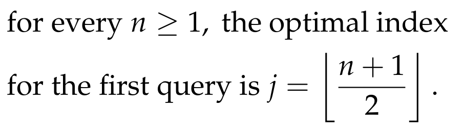
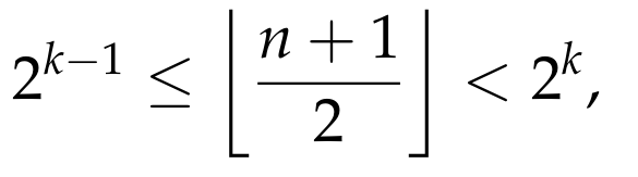
The above imply that the optimal position to query is

and so, if T(n) denotes the number of queries of an optimal deterministic strategy on a list of size n, then we conclude that

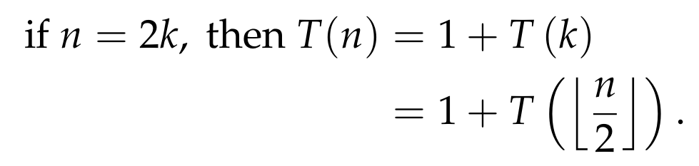
Doing a similar analysis when n=2k is an even number, for some k ≥ 3, we get that:

• j = 1. We have T(n) = 1 + T(2k-1).
• j = 2. We have T(n) = 1 + T(2k-2).
• …
• j = k-1. We have T(n) = 1 + T(k+1).
• j = k. We have T(n) = 1 + T(k).
• j = k+1. We have T(n) = 1 + T(k).
• j = k+2. We have T(n) = 1 + T(k+1).
• …
• j = 2k. We have T(n) = 1 + T(2k-1).

The above imply that the optimal position to query is

which further implies that

Putting everything together, we conclude that

And this is exactly what the famous Binary Search algorithm is doing. At every step, it queries the “mid-point”, and depending on the result of the query, it discards half of the array and continues with the remaining half, as described above.

We will now compute a closed-form expression for T(n).

Calculating the number of comparisons made in the worst case

As shown in the previous section, we have the recursive formula

Intuitively, since the input size reduced by a factor of 2 per iteration, we expect that the function will have a logarithmic behavior. And this is indeed the case. We will show, by using induction, that

(In case you need to refresh you knowledge on Mathematical Induction, you can check the Wikipedia article, or an article of mine on the topic, or the countless many sources available online).

For n = 1, 2,3, it is easy to see that the equation holds. Suppose now that the equation holds for every list of size up to n, for some n ≥ 3. We will show that it holds for every list of size n+1. Since n+1 ≥ 4, we have

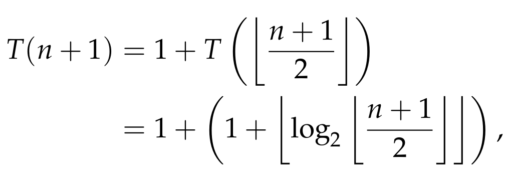
where we used the induction hypothesis, since

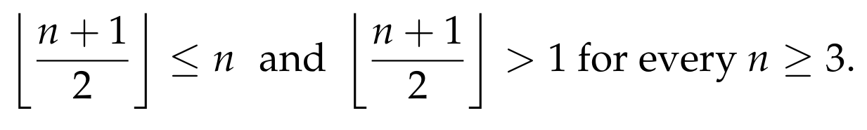
To finish the proof, we will now show that for every n ≥ 3, we have

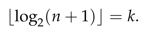
It is easy to see that if n + 1 = 2ᵏ, for some k ≥ 2, then the above equation clearly holds, as both sides of the equation are equal to k. So, we now assume that for some k ≥ 2, we have

This means that

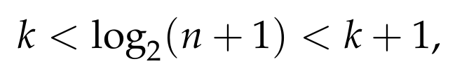
since the log function is strictly increasing. Thus, the right-hand size of the equation that we are trying to prove is

Moreover, we have that

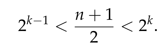
This means that

which further implies that

We conclude that

Thus, both sides of the equation are equal to k, and so the equation indeed holds. This finishes the induction step and the proof.

Comparing the performance of Linear and Binary Search

In order to get a sense of the vast improvement in the running time that we achieved with Binary Search, here are some numbers that hopefully will show how much faster it is compared to Linear Search.

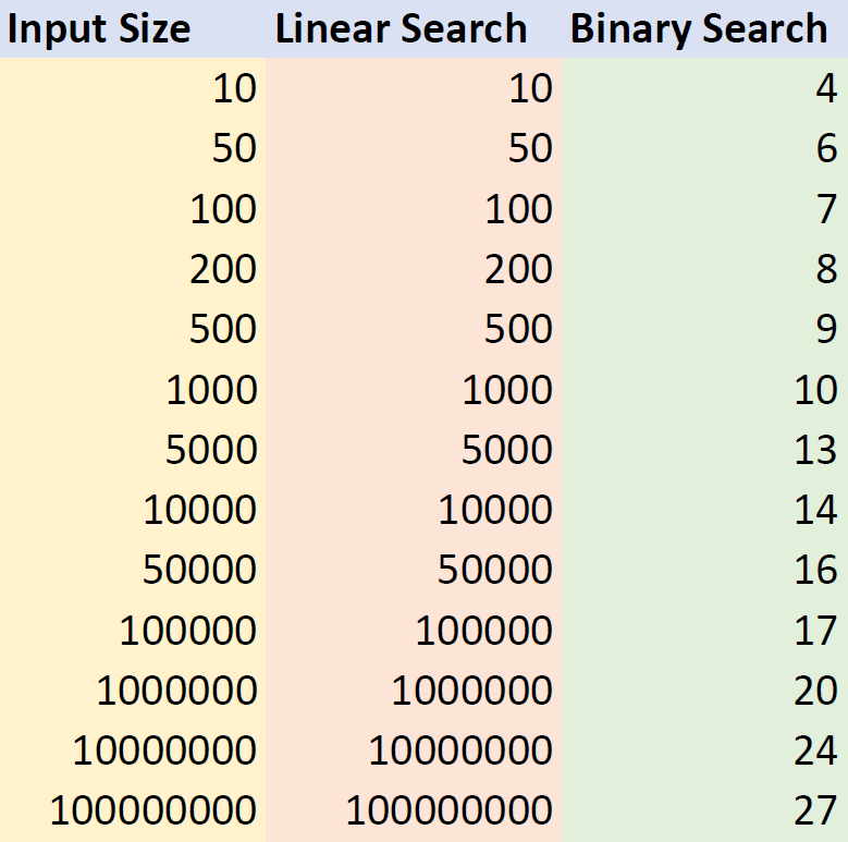
For example, for a list of size 1M, Linear Search might make up to 1M comparisons in the worst case, while Binary Search is guaranteed to make at most 20 comparisons in the worst case. Similarly, for a list of size 100M, Linear Search might make up to 100M comparisons while Binary Search will always makes at most 27!

Implementing Binary Search

We now give a straightforward recursive implementation of Binary Search in pseudocode. The function takes as input a list L of natural numbers (indexed as L[1], L[2], …) and a natural number t, and either returns a position in which tappears in or returns “NO” in the case where t is not in the list L.

We clarify that, due to the recursive nature of the implementation, and since we would like to get the index of the original list L which t appears in, the function has an auxiliary variable offset that is a natural number and is used for this purpose. Since this variable is only used in the recursive calls, the original call is done by setting this variable to 0, i.e., as follows:

BINARY_SEARCH(L, t, 0);

1. BINARY_SEARCH_REC(L, t, offset):
2.
3. int mid;
4.
5. if (|L| == 0)
6. return "NO";
7.
8. if (|L| == 1)
9. if (L[1] == t)
10. return offset + 1;
11. else
12. return "NO";
13.
14. mid = (|L| + 1) div 2;
15.
16. if (L[mid] == t)
17. return offset + mid;
18. else
19. if (L[mid] > t)
20. L' = L[1,...,mid-1];
21. return BINARY_SEARCH(L', t, offset);
22. else
23. L' = L[mid+1,...,|L|];
24. return BINARY_SEARCH(L', t, offset + mid);

We now give a non-recursive implementation of Binary Search, as it is faster, and also highlights one “issue” that many Binary Search implementations have.

1. BINARY_SEARCH_NON_REC(L, t)
2.
3. int i;
4. int j;
5. int mid;
6.
7. i = 1;
8. j = |L|;
9.
10. while (i < j):
11. mid = i + (j - i) div 2;
12. if (L[mid] == t)
13. return mid;
14. else
15. if (L[mid] > t)
16. j = mid - 1;
17. else
18. i = mid + 1;
19.
20. if (L[i] == t)
21. return i;
22. else
23. return "NO";

A few comments about the pseudocode above. The first is about line (9). There, instead of computing (i+j) div 2, as implied by the discussion above, we instead compute i + (j-i) div 2. It is easy to verify that these quantities are equal. Still, there is a reason for our choice. Although the two expressions are equal, if we use the first one, we run into the danger of an overflow, as the number i+j might be very large to represent for our computer. This is a common “mistake” in many non-recursive implementations of binary search that should be given more attention. A second comment is about the final step, at line (18). If we have reached that point, it means that at this point, we have i ≥ j. We now do some case analysis.

• If j is equal to i, then the only position left to check is indeed the one with index i.
• if j < i, this means that at the last iteration of the while loop, we either had mid = i and then we set j = mid-1, or we had mid = j and we set i = mid+1. It is not hard to see that during all the iterations of the while loop, we have mid < j. Thus, the only possibility is the first one, i.e., mid being equal to i, and then setting j equal to mid-1. For this to happen, we must have had that at the beginning of the last iteration, i and j were consecutive integers, and moreover, we must have that L[i] > t. Thus, we can already safely conclude that t is not in the list, and this is indeed what our algorithm will conclude after line (18).

We conclude that the above is a valid implementation of the Binary Search algorithm.

Did we oversimplify things?

So far, the whole analysis we did was based on a unit of cost being a “comparison”, as defined in the introductory section. In particular, we analyzed the complexity of our algorithms by simply counting the number of comparisons that the algorithms are making. Clearly, this is a simplified model of computation. So, it is natural to ask whether it is good enough or whether it oversimplifies the analysis, and thus, resulting in running times that are not accurate.

It turns out that the above analysis is good for most purposes. Unless we are dealing with very large numbers (e.g., numbers that require |L| bits for the representation), we do not lose much by assuming that comparing two numbers takes 1 unit of time. Moreover, all other operations that are executed at each iteration (or, each recursive call) are constantly many and elementary (e.g., incrementing a counter variable by 1), and, so, this means that our analysis is indeed tight up to a constant factor.

To sum up, for all practical purposes, claiming that the running time of Binary Search is O(log |L|) is precise enough and will almost always correspond to the actual running time of our implemented algorithm.

Is Binary Search optimal?

It turns out that we cannot hope for algorithms with running time o(log |L|), i.e., algorithms with running time significantly better than Binary Search. As was already discussed in previous sections, a deterministic comparison-based algorithm (i.e., an algorithm that knows nothing about the input and is only allowed to make a query at some position of the list) will have a recursive structure, like Binary Search, and Binary Search is the optimal such algorithm, as proved above.

We will now give another proof of the fact that Binary Search is optimal, by utilizing Decision Trees, a very useful technique when it comes to discussing lower bounds of deterministic algorithms. A Decision Tree is simply a tree that describes the sequence of comparisons that an algorithm makes. Since each comparison has 3 possible outcomes, each vertex of the tree will have 3 children. Pictorially, a Decision Tree for an algorithm solving our problem looks as follows.

Each black vertex denotes a query at some position j. Depending on the outcome of the query (denoted with red), the algorithm continues with the next query, or stops if the target is found (denoted with the green box).

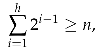
Given a list L of n distinct numbers, every element of the list must appear as a green box somewhere in the tree (since the target element is allowed to be anything, and thus, it is allowed to be equal to L[j], for each j = 1, …, n). It is easy to see that any Decision Tree can have at most 1 green box at the 1st level (the level after the root), at most 2 green boxes at the 2nd level, at most 4 boxes at the 3rd level, and in general, at most 2ⁱ green boxes at level i. Thus, if the tree has hlevels, we must have

which implies that

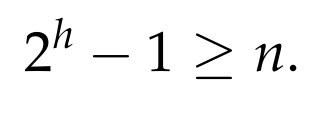
This gives

We conclude that any Decision Tree must have depth at least log |L|, or, in other words, any algorithm must make at least log |L| queries in the worst case.

Conclusion

In this article we discussed one of the most fundamental and widely applied algorithms that is known as Binary Search. The core idea of Binary Search is quite simple, but do encourage the interested reader to try to understand the theoretical analysis of the algorithm, as well as implement it in their favorite programming language. After all, let’s not forget what Donald Knuth has famously said about Binary Search.

“Although the basic idea of binary search is comparatively straightforward, the details can be surprisingly tricky…” — Donald Knuth

References

• https://en.wikipedia.org/wiki/Binary_search_algorithm