The Physics of Superfluidity

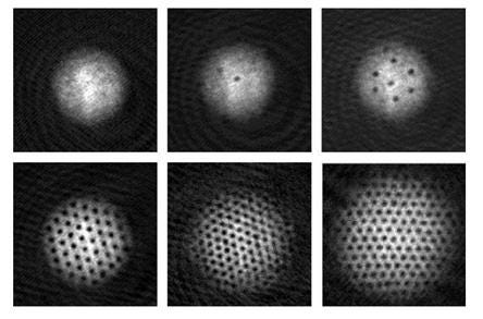
Superfluidity is a property of some fluids to flow apparently without any viscosity (with constant kinetic energy). Examples of superfluids include helium-3 (or ³He) and helium-4 (or ⁴He). For temperatures below 2.17 K, helium-4 becomes a superfluid. Helium-3 becomes a superfluid only below 0.0025 K. Also, when superfluids are stirred, they form vortices that “rotate indefinitely” (see Fig. 1). The appearance of the superfluid phase in ⁴He, which is a boson, is related to Bose condensation, where a macroscopic fraction of the atoms occupies the lowest-energy state. The mechanism that generates the superfluid behavior in ³He is different since ³He is a fermion and the Pauli principle forbids more than one fermion to occupy the same state. Superfluidity occurs in ³He via the formation of pairs of fermions, which behave like bosons (Cooper pairs).

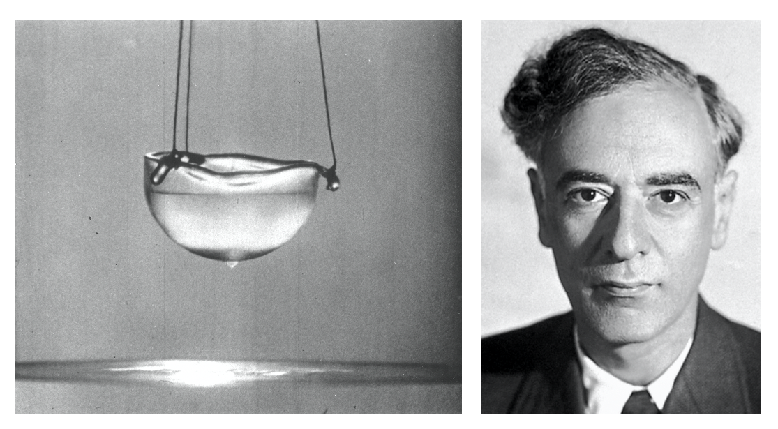
Superfluids also exhibit the so-called fountain effect: recipients containing superfluids empty themselves spontaneously. Fig. 2 shows a superfluid creeping up a cup’s wall as a thin film and coming down on the outside, forming a drop. After the drop falls into the liquid below, a new one will form. The process continues until the cup is empty.

Superfluidity was first discovered by the leading Soviet physicist and Nobel laureate Pyotr Kapitsa and the Canadian-born physicist John F. Allen. The mathematical theory of superfluidity was developed by renowned Soviet physicist and Nobelist Lev Landau.

This article is based mostly on Zee and Lancaster and Blundell. I will follow both and use quantum field theory in the nonrelativistic limit (the analysis can be also done using Bogoliubov transformations) to derive the results.

Warm-Up: The Klein Gordon Field

In the Lagrangian formulation of classical mechanics, a particle is idealized as a point of mass m. Now, suppose its position at some time t is given by x(t) and that the particle moves in a region with potential energy is V(x). Newton’s second law of motion then reads:

The corresponding Lagrangian function L is:

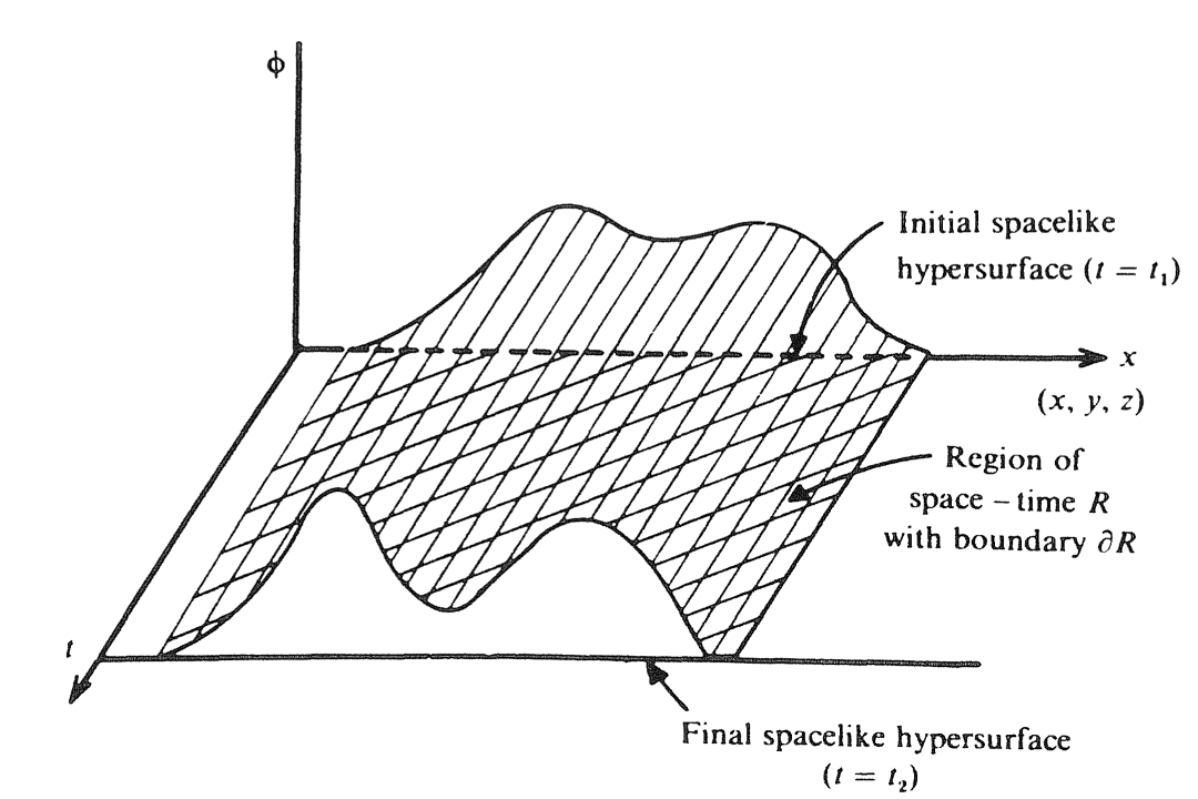
where K and V are, respectively, the kinetic and potential energies. We can envision the passage from a point particle at x(t) to a field Φ(x, y, z, t) as the “replacement” of x by Φ, and of t by (x, y, z). The Lagrangian density has, in this case, the following form:

Note that, Φ is a real scalar field, not a wave function. Eq. 3 is Lorentz invariant (its mathematical form does not change for observers moving with respect to one another within an inertial frame). The scalar field Φ obeys the so-called Klein-Gordon equation:

Complex Scalar Fields

To describe the properties of superfluids we will need to add a layer of complexity to Eq. 3. The Lagrangian density of a complex scalar field is:

This Lagrangian describes interacting bosons. We are specifically interested in the behavior of the slowly moving bosons. For simplicity, let us first find the dynamics of such bosons starting with the equation of motion Eq. 4 for a free scalar field Φ. The solutions of Eq. 4 are modes with the following time dependence:

Since we are interested in the behavior of slowly moving bosons we will write the energy in Eq. 6 as follows:

We can separate the mode given by Eq. 6 into a product of two factors:

Using the approximation:

Eq. 4 becomes the Schrödinger equation:

The nonrelativistic version of the Lagrangian density is obtained by plugging

into Eq. 5 (the prefactor is just for later convenience). After some simple algebra we get:

From the minus sign in the potential term g²ρ², we see that the interaction is repulsive. To avoid the possibility of having zero density in Eq. 10, one usually introduces in L a finite density of nonrelativistic bosons:

The term:

is the Mexican hat or champagne-bottle potential shown in Fig. 4.

A consequence of the form of Eq. 11 is that φ approaches the expectation value of the field φ:

To study spontaneous symmetry breaking we first write φ in polar coordinates:

then add a small perturbation to the expectation value:

Substituting Eq. 15 in Eq. 11 we obtain:

where a total divergence term was dropped. Now, to eliminate h we plug the Lagrangian density into a path integral and integrate it out:

The Lagrangian density becomes:

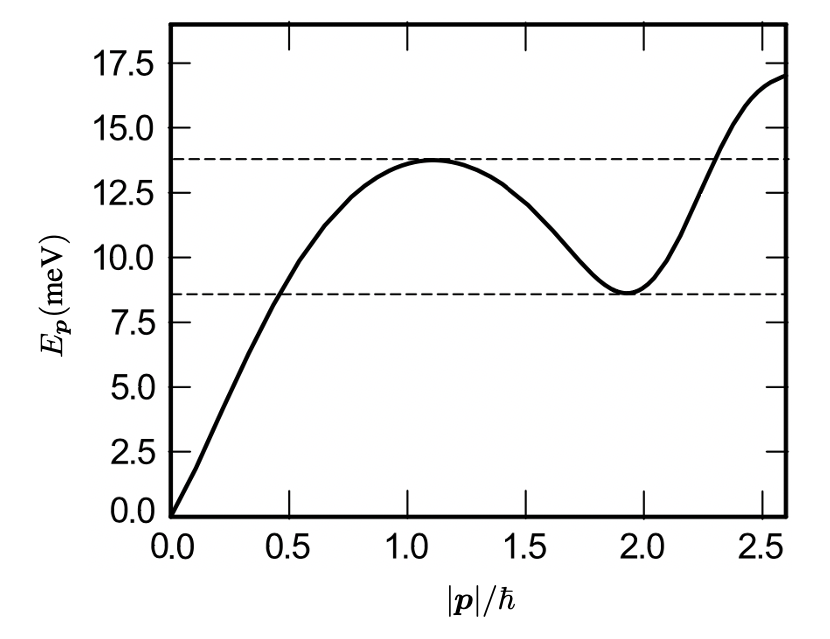
where the spatial derivative in the denominator of the second-hand side of Eq. 17 was dropped. Eq. 15 tells us that there exists a fluid of bosons with gapless mode. The linear dispersion relation (see Fig. 5 below) is given by:

The form of the Lagrangian obtained after spontaneous symmetry breaking gives us the momentum superflow. The massless bosonic field θ is called a Goldstone boson. The presence of Goldstone bosons is a general consequence of the spontaneous symmetry breaking (in Eq. 15).

In Fig. 5 we see the dispersion relation of superfluid liquid obtained experimentally. When the momentum is low, the dispersion relation is indeed linear and at large momentum, the energy goes as p² as we expect for free particles.

Thanks for reading, and see you soon! As always, constructive criticism and feedback are always welcome!

My Linkedin, personal website www.marcotavora.me, and Github have some other interesting content about physics, math and other topics such as machine learning, deep learning, finance, and much more! Check them out!