The Navier-Stokes Equations

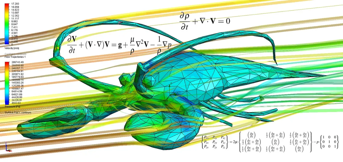
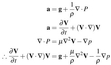
The motion of an incompressible Newtonian fluid with viscosity μ, density ρ, and subject to hydrostatic pressure p and uniform gravity with acceleration g can be described as a velocity vector field V satisfying the Navier-Stokes equations:

The equations are named for Claude-Louis Navier (1785–1836) and Sir George Stokes (1819–1903).

In this first article in my series on the physics of fluids, I will demonstrate the derivation of these equations from first principles.

Preliminaries and notation

The Navier-Stokes equations are differential equations that impose a rule on the velocity V of an infinitesimally small parcel of fluid at every point in space. The result can be interpreted either as the motion of a test particle immersed in the fluid or as the motion of the fluid itself.

We will suppose that the x, y, and z components of V are, respectively, u, v, and w. The unit vectors in the x, y, and z directions will be written x, y, and z.

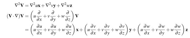
If you’ve had some basic physics or calculus courses, you probably recognize the del operator ∇ and understand what the Laplacian of a scalar function ∇²f and divergence of a vector function ∇⋅F are. There are two vector differential operators in the NSE that may be unfamiliar to you. The first is the vector Laplacian operator ∇²V and the second is the operator (V⋅∇)V. Fortunately, it’s easy to understand what these operators mean. The vector Laplacian applies the Laplacian to each of the scalar components of a vector function, and the second operator applies V⋅∇ to every component:

The basic physics of fluids

A deformation is a process that causes all of the constituent particles of a body of matter to be displaced. We are interested here in continuous deformations, in which the body of matter is not pierced or separated into disjoint parts and in which particles that are infinitesimally close to each other before the deformation are infinitesimally close to each other after.

Deformations of a body of matter are caused by stresses at the surface, of which there are two types. A normal stress has a direction perpendicular to the surface, and a shear stress is parallel to the surface. Stress has units of force/area.

A fluid is defined as a body of matter that cannot resist shear stress. As long as a shear stress is imposed on a body of fluid, the body will continuously deform. This gives rise to the popular definition of a fluid as matter that always takes the shape of its container. A Newtonian fluid is a fluid for which the rate of change of the deformation has a linear relationship with the stress.

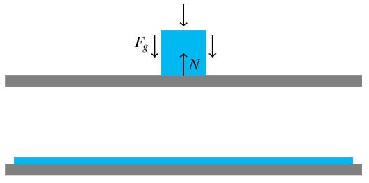
In the above example, the “container” is just a flat surface and the body of water starts out as a cube. There are normal stresses at the top and bottom due to gravity and the normal force from the table and shear stresses at the side due to gravity. The fluid cannot resist the shear stress so to reach equilibrium it will eliminate the shear by making its sides as small as possible. The fluid will spread out over the flat surface, taking on the same shape as its “container”. Surface tension will eventually dominate and prevent the fluid from spreading itself any thinner. The only stresses left will be the normal stresses due to gravity at the top and normal force at the bottom, which will cancel each other out when the fluid is at equilibrium.

Let us now consider a cube-shaped parcel of fluid with its faces normal to the axes. The stress component Pᵢⱼ is the stress on the face perpendicular to i∊{x,y,z} in the direction of j∊{x,y,z} and it will be positive if it points in the +j direction. For example, Pₓₓ is the stress on the face perpendicular to x in the direction of x. The Pᵢⱼ are assumed to be constant on the surface of a parcel.

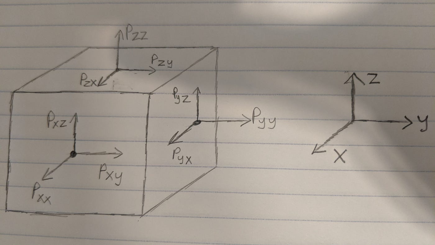
The Pᵢⱼ terms can be arranged into an array called the stress dyadic:

The definition of a Newtonian fluid can therefore be understood as telling us that the rate of change of the deformation is represented by a dyadic E, called the strain rate dyadic, related to P by P=aE+bI where a and b are constants and I is the unit dyadic:

We will identify E precisely in the derivation section.

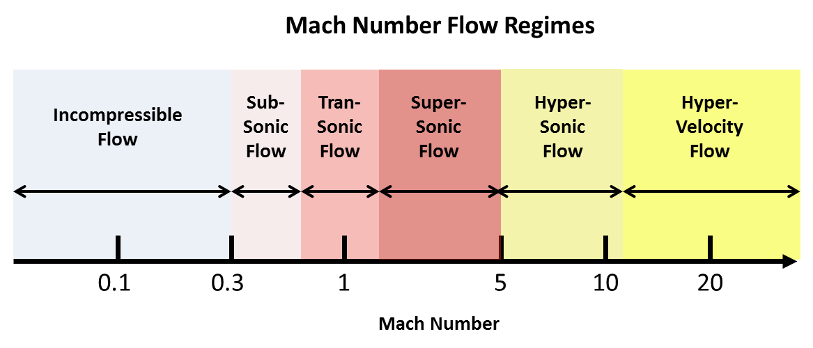
The density ρ is the mass of an infinitesimally small parcel of fluid. An incompressible fluid is one in which the density is constant in space and time. Incompressibility is an accurate approximation for liquids and gases where the speed is less than 30% of the speed of sound in the fluid. Since it’s very difficult to achieve speeds this great in liquid, the study of compressible flows is mostly concerned with gases.

The terms “incompressible fluid” and “incompressible flow” mean different things. An incompressible fluid is one that cannot be forced to change its density, whereas an incompressible flow is one in which the density of the fluid does not change. While all flows involving incompressible fluids are incompressible, it is possible for flows of compressible fluids to be accurately described by incompressible flow under the right conditions. This makes sense because in reality all fluids are compressible.

The viscosity μ measures a fluid body’s resistance to deformation. For a parcel with higher μ, it will require more stress to produce the same deformation in the same amount of time compared to a parcel with lower μ. For example, when water is poured onto a surface it very quickly spreads out, but the same volume of tar will take much longer to cover the same area.

The last term in the NSE is the hydrostatic pressure p. By definition, the hydrostatic pressure of a fluid on a closed surface immersed in the fluid is the average of the normal stress over that surface. Hydrostatic pressure is defined to be positive when it compresses a parcel. Since the Pᵢⱼ are constant on the surface of a parcel, the hydrostatic pressure on a cube-shaped parcel is:

Fluids are subject to the continuity equation:

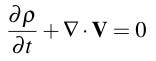
The divergence of V tells us the net flow of fluid into or out of every point and is positive when there is a net outflow, so the continuity equation says that the rate of change of the mass of fluid at a point is equal to the rate of fluid flow into that point. Incompressible flows are divergenceless because ∂ρ/∂t=0.

Digression on tensors

Dyadics belong to a class of objects called tensors. Tensors encode geometric relationships and can be thought of as similar to vectors but more general. For example, a position vector is a tensor that tells you where a point is relative to some choice of origin. The cross product A✕B is a tensor that tells you the normal vector of the plane containing the vectors A and B.

The precise geometric nature of the P and E tensors is not something that we will need to know in this article. The purpose of this digression is to explain how to take the dot product of a vector with a dyadic, which we will need to do later.

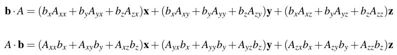
As a mnemonic, we can think about expanding a dyadic in the following form:

The objects xx, xy, etc, can be thought of as products of unit vectors. Each factor obeys the rules for dot products of unit vectors, however they are not commutative. For example, x⋅xz=(x⋅x)z=z but xz⋅x=x(z⋅x)=0. Therefore:

Deriving the Navier-Stokes equations

We start with Newton’s Second Law for an infinitesimal fluid parcel F=ρa. Let’s start by writing down the acceleration.

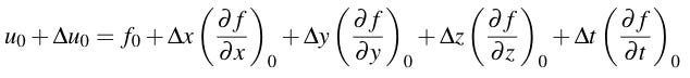
Let u=f(x,y,z,t) be the x-component of the velocity of a test particle immersed in the fluid as it follows the path (x(t), y(t), z(t)). Suppose that the velocity changes from u to u+Δu in time Δt. Then u+Δu=f(x+Δx,y+Δy, z+Δz,t+Δt). By making a linear approximation around the point (x₀, y₀, z₀) at time t₀:

Substitute u back in for f and cancel u₀ from both sides, and then divide through by Δt:

Now take the limit as Δt→0, and recall that u=dx/dt, v=dy/dy, w=dz/dt, and V=(ux+vy+wz). Then the following is true everywhere:

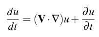
By doing the same for the other components of the velocity, we find that:

This gives us one side of the Newton’s Law equation. Now we need to find the forces.

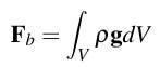
There are two types of forces that act on a body of fluid: body forces and surface forces. Body forces act directly on each particle in the fluid. In practice, the body force is almost always uniform gravitation so the total body force is:

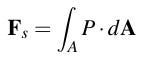
Surface forces interact with the surface of the fluid. The total surface force is by definition the surface integral of the stress tensor:

Fortunately, Gauss’s divergence theorem still applies for dyadics, so:

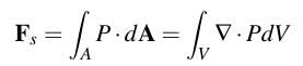
Therefore:

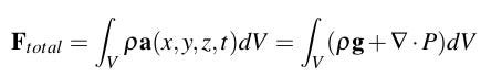
By cancelling the integration we obtain Cauchy’s equation of motion:

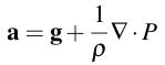
Now we need to compute ∇⋅P. Recall that P=aE+bI where a and b are constants. Stokes found experimentally that a=2μ. Now we need to find the strain rate dyadic.

We start our search with the empirical fact that there are three components to the motion of a fluid parcel: a translation component that represents the parcel moving from one point to another, a component that represents rigid rotation of the parcel, and a deformation component representing the relative motion of two test particles embedded in the parcel.

Consider the velocity V(x,y,z) of a test particle at point (x,y,z) close to a particle with known velocity V₀ located at (x₀,y₀,z₀). We will represent the components of V(x,y,z) as linear approximations near (x₀,y₀,z₀).

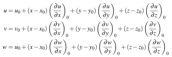
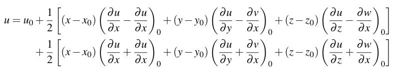
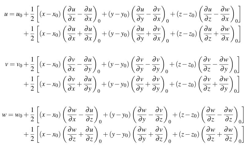
Let’s expand these into a more useful form by adding and subtracting identical derivatives.

By rearranging, we find that:

Similarly for v and w:

We can write this in a simplified vector form if we make the following assignments:

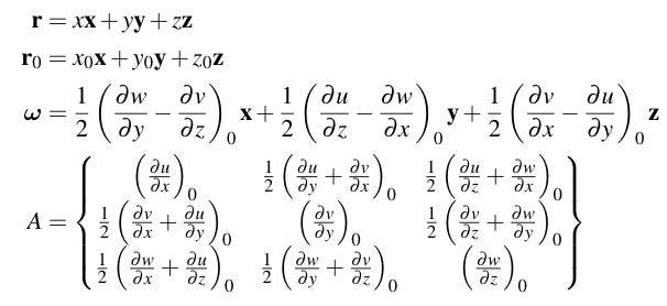
Then we find that:

The first term is constant so it represents translation. The cross product in the second term and the form of the ω vector indicate that the second term is the rotational part. This means that the last part must be the deformation part: it tells us the rate of change of the position relative to r₀ of a particle located at rdue to the deformation of the fluid parcel containing r and r₀. Therefore we can identify A with the strain rate dyadic:

All that’s left is to evaluate b. Although dyadics aren’t really matrices, we can momentarily pretend that they are and take the trace of both sides of P=2μE+bI:

(EDIT: Instead of saying “pretend that they are”, we should really instead say that we’re taking the trace of the matrix representation of this tensor, which is valid for dyadics but not for all kinds of tensors).

Incompressible fluids are divergenceless so b=-p. Therefore P=2μE-pI. Now we can compute ∇⋅P from Cauchy’s equation. By using the procedure in the previous section for computing the dot product of a dyadic with a vector, we find that ∇⋅P=μ∇²V-∇p. Now we obtain the Navier-Stokes equations by substituting everything back into Cauchy’s equation: