This post is about a beautiful result in the field of dimensionality reduction. It is arguably one of the most impressive and satisfying statements about dimensionality reduction in Euclidean spaces. It is named after the mathematicians who proved it in 1984, William B. Johnson (1944-) and Joram Lindenstrauss (1936–2012).

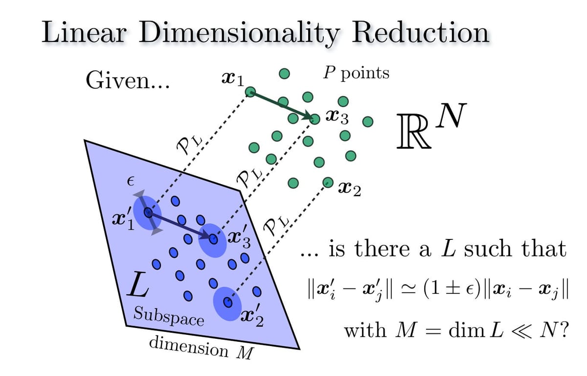
Informally, the lemma says that, given N points with N coordinates each (i.e., these points are in the N-dimensional Euclidean space), we can map these points into a much smaller Euclidean space (in particular, of logarithmic dimension) such that the pairwise Euclidean distances of the given points are preserved up to a multiplicative factor of 1 + ε.

Or, even more informally, if you have N points with N coordinates each, you can always find N new points with roughly log N coordinates each, such that pairwise distances are preserved up to a small constant factor.

If you are a Computer Scientist, you can immediately start thinking about its consequences. For example, an explicit description of the original N points takes space Ω(N²), even when assuming that the space needed to store each coordinate is constant. Storing all pairwise distances also requires Ω(N²) space. But, in the reduced space of logarithmic dimensions implied by the lemma, the total space needed to store an explicit description of all the points is Ο(N log N). This is a significant improvement!

To give a more concrete example, there are many applications where pairwise distances between points need to be recovered multiple times. In an ideal world, we would precompute all pairwise distances and store them in an N² sized table, and then we would be able to recover any such distance in O(1) time; in such case, we would be optimal! But, often N might be of the order of tens of millions or even billions. In such cases, we most likely cannot afford to always maintain such a huge table. On top of that, even the original description of the points is costly, as we do require an N² table just to store the coordinates of the points. So, to sum up, without the JL lemma, there are 2 possibilities:

1. Store the table of points and the table of pairwise distances, and maintain both tables in our memory as long as the application is “running”.
2. Store the table of points, but decide to compute distances on the spot, whenever requested. Each computation would take time Θ(N) in this case.
3. Compute this new set of N points, and store their coordinates in a table of size Θ(N log N). Then, whenever needed, compute the distance of two points on the spot, a task that now requires O(log N) time.

The third option seems to be the most reasonable. We end up using almost linear space, instead of quadratic, and each computation now takes logarithmic time, which is an exponential improvement compared to the linear time needed in option (ii). The only “catch” is that we have to be willing to introduce a small error in our results, meaning that the distances we compute might be off by, say, 1%.

This is some of the strength of the Johnson-Lindenstrauss Lemma!

Before proceeding with some discussion on the proof of the lemma, I quote a nice response from the cstheory.stackexchange about the applicability of the JL lemma compared to the Singular Value Decomposition (SVD), in case some of you already have such questions. If you don’t know what SVD is, then feel free to skip to the next section.

When to use the Johnson-Lindenstrauss lemma over SVD?

Proving the Johnson-Lindenstrauss Lemma

We will now go ahead and say a few things about its proof. We will not provide a formal proof, as there are many sources online providing it, so we will just explain what is the main key lemma needed in order to obtain the result.

We first give the formal statement. We note that this is indeed a proper theorem, but for historical reasons, we still call it a lemma!

We do stress here that the JL Lemma is tight in terms of the dependence of K on N and ε. The tightness of the lemma has settled quite recently by Kasper Green Larsen and Jelani Nelson (2017).

Again, we resort to randomness. The original proof of the Lemma essentially goes as follows: pick a random K-dimensional linear subspace and then take the orthogonal projection of the points on it. That simple! Then, one can show that with strictly positive probability, all pairwise distances are preserved up to this 1 + ε factor. Thus, a linear map that satisfies the desired properties must exist. (Thanks again to the Probabilistic Method! [Shameless plug follows] In case you have missed it, I have written two short articles about applications of the Probabilistic Method that can be found here and here).

One way to construct such a random linear projection is by using Gaussian random variables. More formally, one can prove the following lemma.

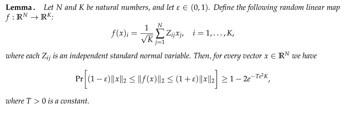
The above lemma says that this random linear map is an “almost isometry” (i.e., it almost preserves the length) for a given vector x. The proof is based on concentration properties of the Gaussian distribution; a very nice exposition of the proof is given in the “Lecture notes on Metric Embeddings” by Jiri Matousek.

Once we have the above lemma, then we are essentially done. To see this, we now explicitly set the parameter K in the JL Lemma to be equal to

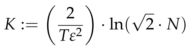
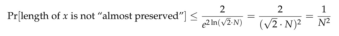
With such a choice of K, the above lemma states that for a vector x, the probability that its length is not “almost preserved” is

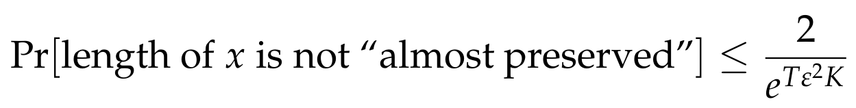
Let’s focus on the exponent of the denominator. We have

Plugging this value back to the previous inequality, we conclude that

We now consider what the above lemma implies about the vectors

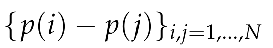
The above lemma implies that for given i, j,

In total, we have

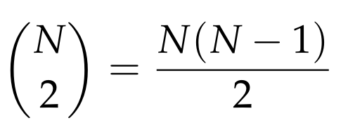
such vectors whose distances we want to preserve. Thus, by applying the Union Bound we conclude that the probability that at least one such distance is not “almost preserved” is at most

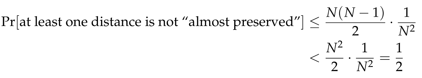
We conclude that with probability at least 1/2, all pairwise distances are almost preserved! And since the map f is linear, which means that

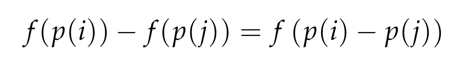
we can simply consider the N points

and we are done!

Note: it is easy to get the correct value of the constant C in the statement of the JL Lemma above by switching from ln to log and taking care of the resulting constants showing up in the above expression of K.

Conclusion

A few concluding comments:

• We stress that the random map we used is linear, which makes it easier to analyze.
• We also mentioned that the result is tight, and this applies to non-linear maps as well. In other words, no matter what crazy non-linear map you consider, the parameters of the JL Lemma cannot be improved!
• The probability of success can be boosted by simply repeating the “experiment” a few times. Thus, the above proof is constructive, in the sense that we can compute such a map with high probability!
• There are other proofs of the JL Lemma. A particularly interesting one is the proof of Dimitris Achlioptas (his paper can be found here), that shows that one can use a random projection matrix that only has {-1, 0, 1} entries. In other words, coin flips (biased in this case) can actually do the trick!