The Heat Equation: Inhomogeneous Boundary Conditions

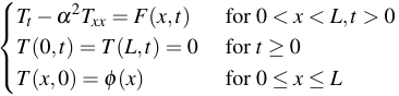
Last time, we looked at IBVPs for the heat equation in which forcing was present and the boundary conditions were homogeneous.

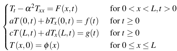
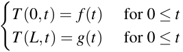
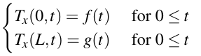
This article will cover how to solve IBVPs for the heat equation with more complicated boundary conditions, in which the problem has the form:

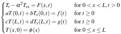
In this problem, f(t) and g(t) are smooth functions, meaning that they are continuous and have continuous derivatives to all relevant orders, and a, b, c, and d are constants.

General solution

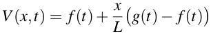
Suppose that T(x,t) has the form T(x,t) = U(x,t)+V(x,t) where V is a smooth function that satisfies only the boundary conditions:

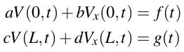
We will assume that V has the following form, since the constants can be chosen so that it will satisfy these conditions:

Now let’s substitute U+V into the IBVP for T:

By making the substitutions G=F-Vₜ+α²Vₓₓ and φ(x)=ϕ(x)-V(x,0) we see that the function U=T-V satisfies the following IBVP with homogeneous boundary conditions:

Now the boundary conditions are homogeneous and we can solve for U(x,t) using the method in the previous article. The presence of the first derivative Uₓ in the boundary condition does not impact the suitability of that method.

The function U(x,t) is called the transient response and V(x,t) is called the steady-state response. Physically, we interpret U(x,t) as the response of the heat distribution in the bar to the initial conditions and V(x,t) as the response of the heat distribution to the boundary conditions.

Dirichlet boundary conditions

Dirichlet boundary conditions, named for Peter Gustav Lejeune Dirichlet, a contemporary of Fourier in the early 19th century, have the following form:

In the context of the heat equation, Dirichlet boundary conditions model a situation where the temperature of the ends of the bars is controlled directly. For example, the ends might be attached to heating or cooling elements that are set to maintain a fixed temperature. Note that this means that b=d=0 and not that Tₓ(0,t) and Tₓ(L,t) are explicitly zero.

The steady-state response is:

To demonstrate, let’s modify a problem that we solved in Part One by making T(L,t)=50°C instead of 0°C.

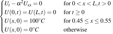
So the steady-state part is V(x,t) = 50x. There is no forcing and Vₜ=Vₓₓ=0 so G(x,t)=0, so the IBVP for the transient response is:

We’ve solved this problem before so we already know the Fourier coefficients:

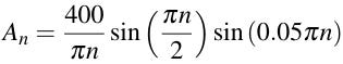
Therefore the solution to this IBVP is:

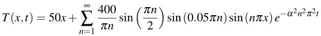
In the animation of the solution, you can see that the solution for U(x,t) vanishes and the solution converges to 50x as t increases:

Neumann boundary conditions

Neumann boundary conditions, named for German mathematician Carl Neumann, have this form:

In the context of the heat equation, Neumann boundary conditions model a situation where the rate of flow of heat into the bar at the ends is controlled. For example, if one of the ends is insulated so that heat cannot enter or leave the bar through that end, then we have Tₓ(0,t)=0. As before, this only means that a=c=0 and not necessarily that T(0,t) and T(L,t) are explicitly zero.

For Neumann boundary conditions, the steady state solution has the following form:

One thing to be aware of when Tₓ appears in the boundary conditions is that Tₓ is proportional to the gradient of the heat distribution, since Q=cT where c is the specific heat capacity. Recall that the second law of thermodynamics says that heat flows in the direction in which the temperature distribution decreases most quickly. In one dimension, this means that if Tₓ is positive at x so that T increases with increasing x (i.e. to the right) then heat is flowing to the left at x, and vice versa. This means that if Tₓ is positive at x=0 then heat is flowing out of the bar at x=0, and heat flows into the bar at x=0 if Tₓ is negative at x=0, and the opposite is true at x=L.

With all of that in mind, let’s solve the following IBVP:

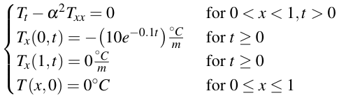
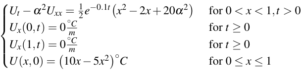
The steady-state response is:

The forcing term in the problem for the transient response is G=-Vₜ+α²Vₓₓ and the initial condition is φ(x)=-V(x,0) so this problem is:

Using the procedure we developed in Part Two, we find that the Fourier coefficients that we need to solve the problem are:

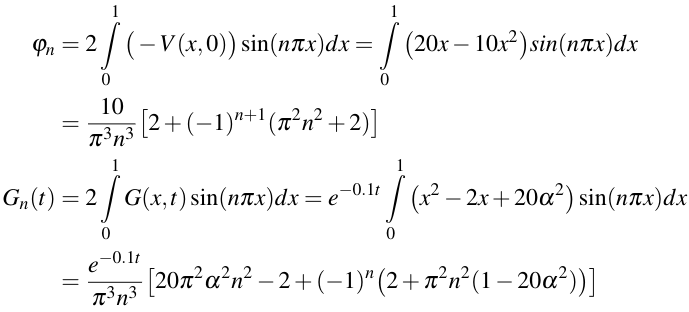
This gives us what we need to solve for U(x,t) and then we find the solution T(x,t) by adding V(x,t).

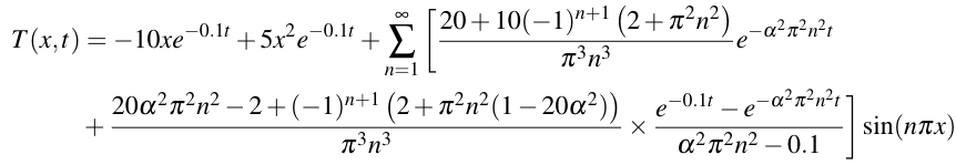
The animation of the solution will probably make more sense:

Mixed boundary conditions

When T and Tₓ both appear in the boundary conditions, we say that they are of mixed type. There is no single formula for V(x,t) in this case and the constants A₁, B₁, etc in the expression for V will need to be solved for on a case-by-case basis. Let’s now consider the following IBVP:

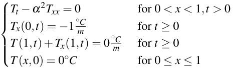
As before, let T=U+V. Let’s plug this in to the boundary conditions to look for V(x,t):

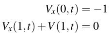
We want Uₓ(0,t)=Uₓ(1,t)+U(1,t)=0 so this means that:

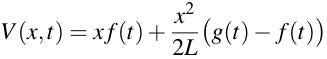
Since f(t) and g(t) are constant, V(x,t) is a quadratic polynomial in x. The solution for V is the polynomial that satisfies the above conditions:

Now we just need to solve the IBVP for the transient response:

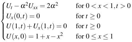
The Fourier coefficients that we need to solve this problem are:

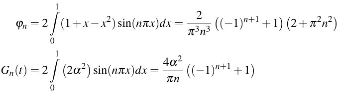
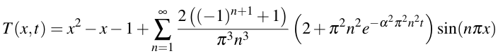
This gives us enough to find the solution, which turns out to be:

Concluding remarks

This ends our discussion of the heat equation, at least for now. At this point we’ve only scratched the surface, without even having considered situations like heat flow in more than one dimension, heat flow with convection, or problems where T appears explicitly in the PDE, such as Tₜ-α²Tₓₓ=aT for constant a. Before we move on to that, let’s put the heat equation aside and continue our survey of the “basic” PDEs of mathematical physics, moving on first to the wave equation and then to Laplace’s equation.