The Heat Equation: Forcing

Last time, we solved some very simple IBVPs for the heat equation in which there was no forcing and T(0,t)=T(L,t)=0°C. These problems had the form:

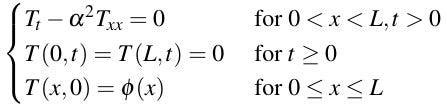
The equation Tₜ-α²Tₓₓ=0 is called the homogeneous heat equation. From now on, we will use α² for the diffusivity instead of k/ρc. A variable in a subscript means a partial derivative with respect to that variable, for example Tₓₓ=∂²T/∂x².

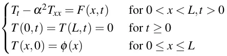
Problems of that type model a long and thin metal bar that was given some initial temperature distribution and was insulated along its length so that it could exchange heat with its surroundings only at its ends. Now we remove the insulation so that the bar can also exchange heat with its surroundings along its entire length. This situation is modeled by an IBVP for the inhomogeneous heat equation:

The function F(x,t) is called the forcing term. For now we’ll keep things simple and only consider cases where the forcing does not depend on the temperature.

General Solution

At every moment of time, the solution T(x,t) is a piecewise continuous function on the interval 0≤x≤L with T(0,t)=T(L,T)=0. From the last article, we know that the set of functions satisfying this condition is a vector space spanned by the basis:

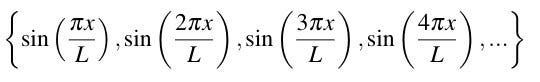
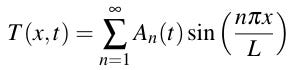
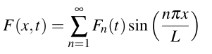
This means that at each moment of time, the solution is a weighted sum of these basis functions. This means that the time dependence of the solution must be contained in the coefficients, so the solution has the form:

The forcing term is also a piecewise continuous function on that domain which satisfies F(0,t)=F(L,t)=0 so it can be expanded in the same way:

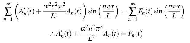
The functions Fₙ(t) are the Fourier coefficients of F(x,t). Here is what we get when we plug these into the heat equation:

This is a first-order linear ordinary differential equation, so it can be solved by the method of integrating factors.

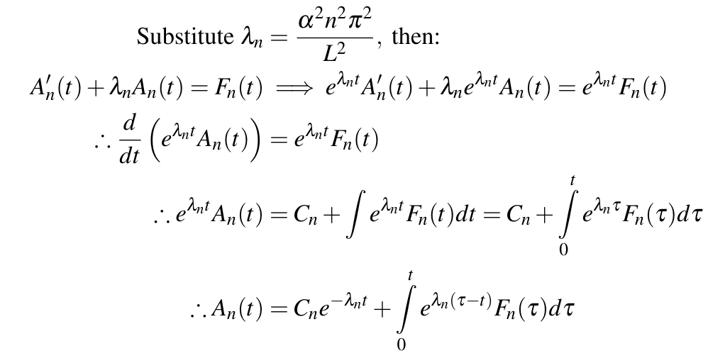
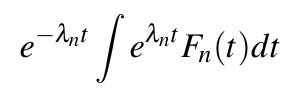
In the fourth line, we replaced the indefinite integral with respect to t with a definite integral over the dummy variable τ from 0 to t. This definite integral will be equal to a function of t minus a constant, and we can assume that this constant is “absorbed” into the constant of integration Cₙ that was picked up when we integrated both sides of the third line. This step is just to avoid a potentially confusing expression with a function of t multiplied by an indefinite integral with respect to t:

If we plug t=0 into the expression for Aₙ(t) we get Aₙ(0)=Cₙ, so the Cₙ are the Fourier coefficients for T(x,0)=ϕ(x) and we will write these as ϕₙ.

Therefore the general solution is:

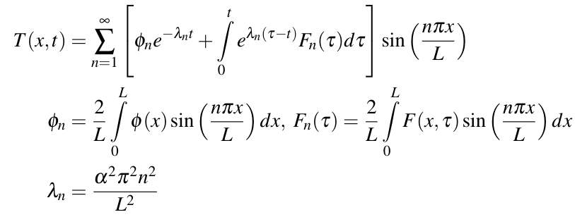
So finding the particular solution to a given IBVP for the inhomogeneous heat equation amounts to simply computing two integrals.

Analytical example: Heating and cooling

This example will cover an IBVP where the forcing and initial and boundary conditions are given by:

The forcing term is animated below. You can see that it will heat and cool different parts of the bar at different times:

Now let’s calculate the Fourier coefficients. Clearly ϕₙ=0, and the forcing function is already in Fourier series form, so F₁(t)=cos(2πt) and F₂(t)=cos(πt) and all others are zero. Then the solution is:

The following graphics assume diffusivity α²=2×10⁻² m²/s.

And here’s the mesh plot:

Numerical example: Forcing defined piecewise

The temperature is initially 0°C throughout the length of the bar and the diffusivity is α²=2×10⁻² m²/s. The insulation has been scraped off of the middle 10cm of the bar and this segment is attached to a heating element that raises the temperature at a constant rate of 5°C/s for 5 seconds and then switches off. For t≤5s, we have:

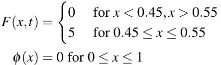
Then for t>5s, we have the new problem:

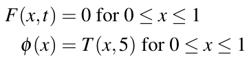
We will solve this problem piecewise. For t≤5s, the solution is found by just plugging F(x,t) and ϕ(x) into the general solution. During this phase, ϕₙ=0 and the Fₙ(t) are constants which will need to be found numerically. Then for the next phase, we solve the homogeneous heat equation using T(x,5) as an initial condition. This will require us to replace t with t-5 since we are basically treating t=5 as a new origin. During this phase, Fₙ(t)=0 and the ϕₙ are the Fourier coefficients of T(x,5), which as before will need to be found numerically.

Here is an animation of the solution:

I used MATLAB to compute and animate the solution. You can get the code here on Pastebin.

Conclusion

In the real world, systems that undergo processes that can be described by the heat equation aren’t perfectly isolated. They interact with the outside world, and this interaction is modeled by the forcing term. Now that we can deal with forcing, we’re a step closer to being able to use the heat equation to model real physical phenomena. However, this article dealt only with the very restricted case of forcing that does not depend on the temperature of the bar. This is unrealistic since in the real world the rate of heat exchange with the environment will depend on T(x,t), for example in the case of Newtonian cooling where the rate of heat exchange at (x,t) will be proportional to the difference between T(x,t) and the ambient temperature, but covering this restricted case was necessary to develop the techniques that we’ll need when we get to more realistic problems.