The genius of Isaac Newton has few parallels in the history of science. His masterpiece, the Philosophiæ Naturalis Principia Mathematica, often referred to as the Principia, is considered one of the most important scientific works in history (see this link). The renowned Indian physicist Subrahmanyan Chandrasekhar, one of the receivers of the 1983 Nobel Prize for Physics, wrote in his essayShakespeare, Newton and Beethoven or patterns of creativity:

“It is only when we observe the scale of Newton’s achievement that comparisons, which have sometimes been made with other men of science, appear altogether inappropriate both with respect to Newton and with respect to the others.”

A Bird’s-Eye View of Kepler’s Laws

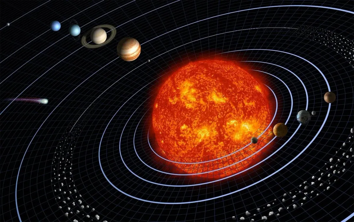
Between the years 1609 and 1619, the German astronomer and mathematician Johannes Kepler published his three laws of planetary motion that describe the orbits of the planets around the Sun.

The laws are:

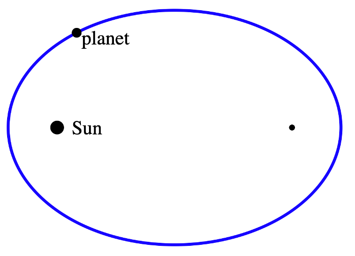
• The orbit of a planet is an ellipse with the Sun at one of the two foci.

• A line segment joining a planet and the Sun sweeps out equal areas during equal intervals of time. The animation below illustrates Kepler’s second law in action. In a fixed time period, the same blue area is swept out. The purple arrow (directed towards one of the foci of the ellipse) is the acceleration. The other arrow is the velocity (the components of the acceleration are also shown).

• The square of a planet’s orbital period is proportional to the cube of the length of the semi-major axis (see Fig. 11) of its orbit.

Halley’s Visit to Newton

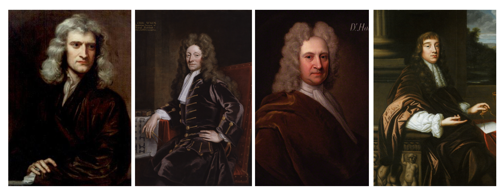
Christopher Wren, the acclaimed English architect, who was also an astronomer, mathematician and physicist, the English polymath Robert Hooke and the English astronomer, mathematician, and physicist Edmond Halley were discussing at a coffee house, after a meeting of the Royal Society, how to prove that the elliptic orbit of the planets was a consequence of the inverse-square force (according to which the gravitational force acting on the planets is inversely proportional to the square of their distance from the Sun). Halley then visited Cambridge to discuss the topic with Newton. The French mathematician Abraham de Moivre later described their meeting:

In 1684 Dr. Halley came to visit him at Cambridge. After they had been some time together, the Dr. asked him what he thought the curve would be that would be described by the planets supposing the force of attraction towards the sun to be reciprocal to the square of their distance from it. Sir Isaac replied immediately that it would be an ellipse. The Doctor, struck with joy and amazement, asked him how he knew it. Why, saith he, I have calculated it. Whereupon Dr Halley asked him for his calculation without any farther delay. Sir Isaac looked among his papers but could not find it, but he promised him to renew it and then to send it him…

Newton’s biographer Gale Edward Christianson, in his book Isaac Newton, describes the events following Halley’s visit:

“[I]n November 1684… eleven months after Halley, Hooke, and Wren… discussion that had started the quest, a copy of De Motu arrived at Halley’s doorstep... [He] was astounded, for in his hands were the mathematical seeds of a general science of dynamics… At first, Newton… thought of De Motu as an end in itself. But once his creative powers were loosed, there was no checking their momentum. ‘Now that I am upon this subject’, he wrote Halley…, ‘I would gladly know the bottom of it before I publish my papers…’ De Motu would serve as the germ of his masterpiece, the greatest book of science ever written. Thus began eighteen months of the most intense labor in the history of science. In April 1686 Newton presented… the first third of his illustrious work. He titled it Philosophiae Naturalis Principia Mathematica…”

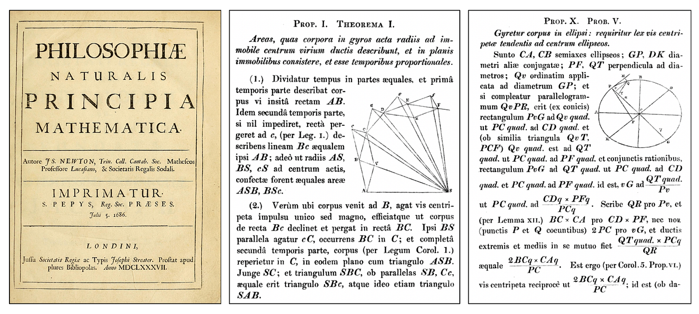
The figure below (containing pages of the Principia) shows excerpts of Newton’s proofs of:

• Kepler’s second law (see above).
• The inverse-square law, according to which the attractive force acting on a planet that is orbiting in an elliptical trajectory around the Sun is proportional to 1/r² and points to one of the foci of the ellipse (this is, in fact, the inverse of the problem described by Halley to Newton).

To visualize the steps taken by Newton to prove Kepler’s second law of planetary motion, the following (slow) animation (Fig. 7) is useful.

A Modern Proof of The Inverse-Square Law

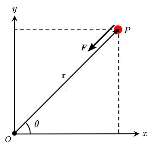
The following analysis follows the book by Symon. Consider the gravitational central force of the sun on a planet. A central force is a force F directed along the line joining an object and the fixed origin O of the force. The goal of this article is to determine the motion of a body acted on by such force (the inverse of the problem proposed by Halley, but which was also solved by Newton).

Some Simple Kinematics in a Plane

The polar coordinates (r, θ) are related to the cartesian coordinates (x, y) by:

The unit vectors in the directions x, y, r, and θ are shown in the figure below.

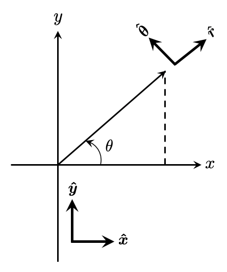
The relations between them are given by:

The position vector is equal to:

Differentiating Eq. 3 twice with respect to time, we obtain, after some simple algebra the acceleration vector expressed in polar coordinates:

Time Evolution of the Orbiting Body

It is straightforward to show that the angular momentum (the rotational equivalent of linear momentum) of a body acted on by a central force is constant:

Since L is constant, the position and velocity vectors, x and v, always remain in a fixed plane (orthogonal to L), substantially reducing the problem’s complexity. Eq. 4, together with Newton’s second law of motion F = ma, give us the equations of motion we want to solve:

Now, if we write the angular momentum as

differentiate it with respect to t, and use Eq. 5 we obtain the second line of Eq. 6. Integrating Eq. 5 we get:

where the constant L depends on initial conditions. Integrating the first line of Eq. 6 and using Eq. 7 or Eq. 8, we obtain:

The total energy E is another constant that depends on initial conditions. Solving Eqs. 8 and 9 for dθ/dt and dr/dt respectively and then integrating, we obtain equations for r(t) and θ(t):

Note that in Eq.10 there are four constants that depend on initial conditions, namely, namely, E, L, r₀, θ₀.

Finding the Trajectory

Finding the exact solutions r(t) and θ(t) of the two equations in Eq. 10 is usually quite tricky. What is more straightforward is calculating the trajectory of the orbiting body, namely r(θ).

First, consider Eq. 6 and Eq. 8 and transpose the term containing L to the right-hand side of Eq. 6. We obtain:

where we defined an effective potential. The two-dimensional problem becomes therefore a one-dimensional problem for r, since dθ/dt was eliminated by Eq. 8.

Defining a new, auxiliary variable u=1/r and substituting it into Eq. 11, we obtain, after a little algebra:

Since we are interested specifically in the gravitational force acting on an orbiting body, F becomes:

Substituting Eq. 13 into Eq. 12 and solving it, we obtain the equation of a conic section, namely:

(recalling that u=1/r). To go from Eq. 12 to Eq. 14, we solved the homogeneous equation, found a particular solution, and then put both together.

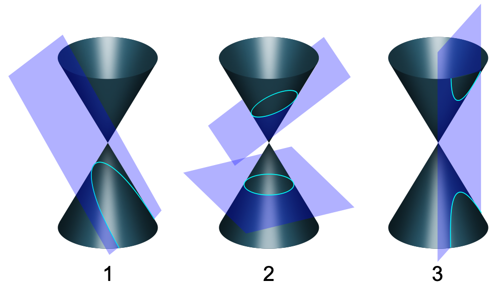
In Eq. 14:

• r=0 is the focus of the conic section
• θ₀ is the orientation of the orbit in the plane containing the curve.
• A is a constant. Since θ₀ is arbitrary we can choose A to be positive.

We are particularly interested here in the elliptical trajectory. It has two turning points corresponding to θ₀=0 and θ₀=π in Eq. 14. From Eq. 9 and Eq. 11, we see that the turning points occur when the effective potential equals the total energy E. Therefore, solving Eq. 11 for r setting the effective potential to be equal to Ewe obtain two equations, one for each turning point, expressed in terms of E and L. Comparing these equations with Eq. 14 for θ₀=0 and θ₀=π we obtain the value of A:

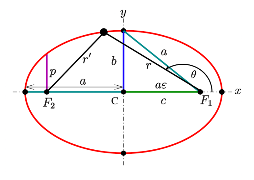
From analytic geometry, we know that the equation of the ellipse in polar coordinates is:

where ε is the eccentricity (the value ε of an ellipse is greater than zero but smaller than 1).

Eq. 14 for the ellipse can be re-written as:

Two important relations obeyed by an ellipse are:

Comparing Eq. 14, and 17 we obtain B in terms of the angular momentum L:

Using ε=A/B we get:

We finally arrive at the equation of the ellipse followed by a body orbiting another body located at one of the foci of an ellipse. It is given by:

Thanks for reading and see you soon! As always, constructive criticism and feedback are always welcome!

My Linkedin profile, my personal website www.marcotavora.me, and my Githubprofile have some other interesting content about physics and other topics such as mathematics, machine learning, deep learning, finance, and much more! Check them out!