The beginner’s guide to proving the Fundamental Theorem of Calculus, with both a visual approach for those less keen on algebra, and an algebraic, slightly more rigorous approach, for those keen on exactness.

By the end, I hope you feel a bit more like a mathematician :)

Introduction, motivation and ‘hello!’

Hello! We are going to understand one of the most historically important and brilliant proofs in mathematics. Important and brilliant because it reduces previously impossible problems — that of integrating functions — into the art of spotting a derivative. But more on that soon.

What is wonderful about this proof is that there are two approaches, both of which complement each other, but also can be understood independently. To begin with, we will see an informal statement of the theorem, and an informal statement of the proof. This will give the intuition and ‘essence’ of what we are doing. This proof will be visual in nature, and not require excessive or complicated algebra. This part will convey some key ideas without algebra, but at the cost of being less exact. Next will come a formal statement and proof. This is optional. Why do I nevertheless encourage you to try and understand it, even if you aren’t very comfortable with ‘algebra’ proofs compared to visual proofs?

1. The visual proof captures the key ideas, but the formal proof shows how mathematicians turn those ideas into mathematical objects and then prove things about the mathematical object
2. Having seen the visual proof, you will have some idea what is going on in the algebra proof even if you don’t follow all the details
3. Ideas in mathematics sometimes take a while to sink in. Taking time to think about something is never time wasted. At some later point the ideas will click, or be handy elsewhere. Time spent thinking about mathematics is fundamentally time well spent. Although, I am somewhat opinionated :)
4. You’ll never know if you never try :)

A (very) short introduction to Derivatives (for those who haven’t encountered derivatives before)

Derivatives are about approximating functions with straight lines. The idea is that, near a point, the tangent line provides a pretty good approximation to how the function is changing.

The derivative of a line at a point can be viewed as the slope of the ‘best’ linear approximation at that point.

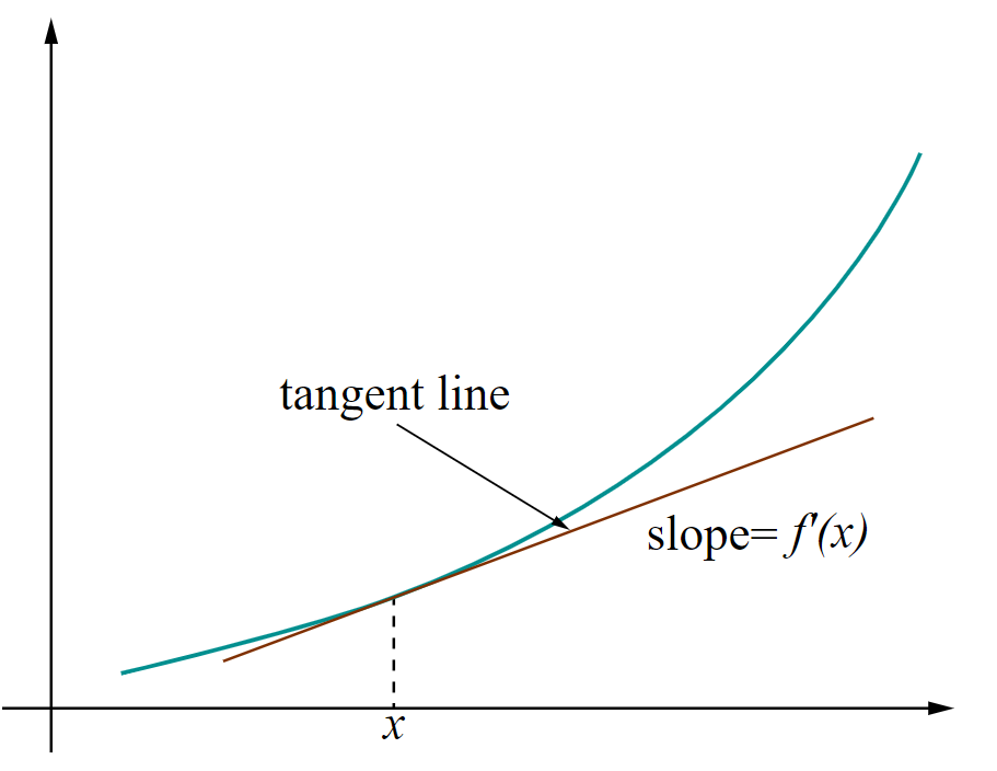
The idea is that, for many functions, a lot of the information about the function is contained in using a linear function to approximate it. Obviously, this approximation isn’t perfect, but if such an approximation holds everywhere, we learn a lot about the function: in fact we can recreate the function upto a constant term.

At the end of the article are some resources on understanding derivatives and other aspects of calculus, if you want to go into greater detail. We will also define the derivative at bit more precisely later.

Part 0: An informal Statement

The Fundamental Theorem of Calculus then tells us that, if we define F(x) to be the area under the graph of f(t) between 0 and x, then the derivative of F(x) is f(x).

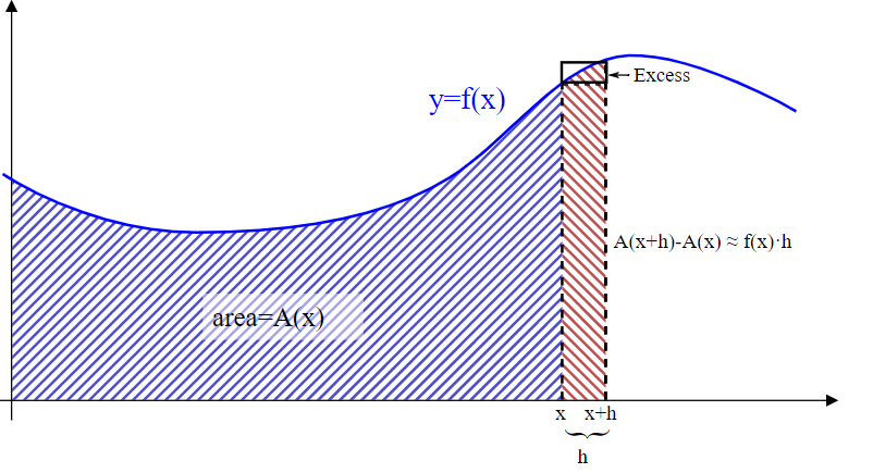
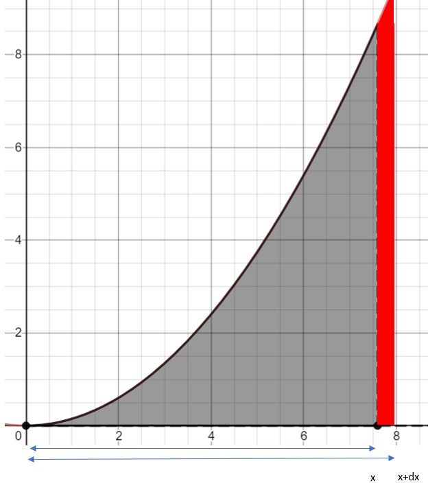
Let’s digest what this means. Below is a red line — this is our function f. We want to find out the area between 0 and x — x is marked red on the x-axis. Our function F tells us, for each point on the x axis, what the area is under the curve at that point. [Please excuse my poorly drawn ‘x’]

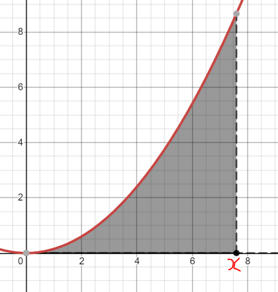
We want to determine what derivative of our function F is — at x. We can get a graphing calculator (I used desmos, but geogebra is also good and free) to plot F(x), which I have done below:

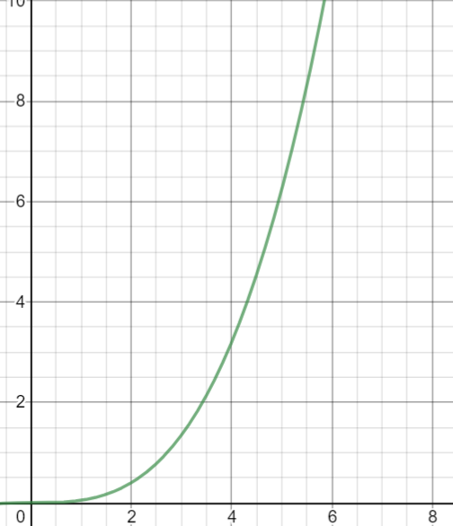
So this function looks like it should have a derivative. But what is it?

Part I: An Informal Proof

Imagine we look at the best line approximation to F(x) close to x. What might this look like? Well, how about we make a good guess.

Let’s suppose F(x+dx) is roughly equal to F(x) + dx*f(x)

For instance, at x = 8, we might say that F(8.00001) is well approximated by F(8) +0.00001*f(8). What is the ‘visual’ proof of this?

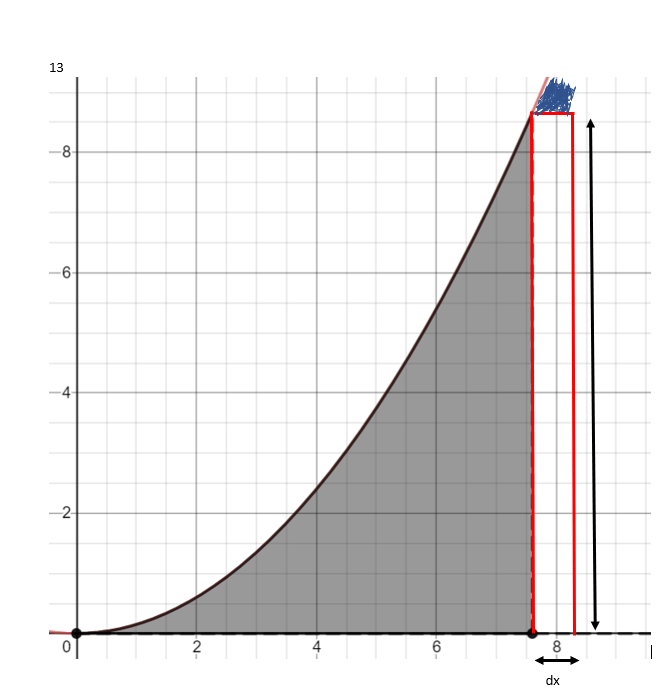
Let’s look at the area under the graph again.

When we use the approximation F(x+dx) roughly equals F(x) + dx*f(x) we see the following. dx*f(x) is represented by the area of the red rectangle, which has height f(x) and width dx. Is this a good linear approximation? Yes! Rewriting, our approximating function at x = 8 is F(8) + h*f(8). We also see that the rectangle contains ‘nearly’ all the area F(x) would have gained by going to F(x+dx). This can be seen below, where the area we ‘missed’ is just the small blue shaded region, which is much much smaller than the rectangular region.

However, there are several improvements we can make on this proof. Yes, it certainly looks like a good approximation on this graph, but does it work on all graphs? After all, graphs can look very different. Also, how are we defining our ‘best linear approximation’? This leads to formulating the problem using some algebra.

Part II: A Statement using Algebra

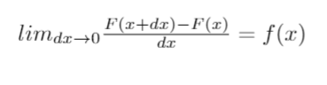
First, we want to define our derivative. This is done as follows:

[‘lim’ stands for ‘limit’]

The limit just means to look at what happens to the expression as dx gets arbitrarily close to 0. So, you might compute the following sequence and see where it ‘tends’ towards

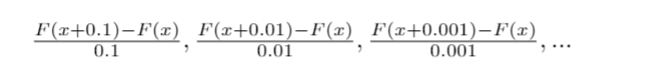
For the functions we’re interested in, it won’t matter which sequence you pick for ‘dx’ , provided it tends to 0.

We get a nice visual feel for it in the following diagram:

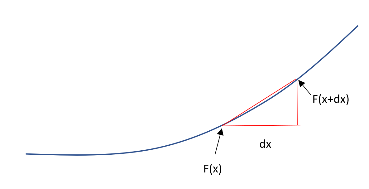
We then see that, as dx tends to 0, the limit of the gradient of the straight line connecting F(x) with F(x+dx) is defined to be our derivative. This can be seen below.

Tangent animation.gifFrom Wikimedia Commons, the free media repositorycommons.wikimedia.org

We use a limit because, while x = 0.01 or 0.00001 may seem small to us, for a function like x¹⁰⁰⁰⁰⁰⁰⁰⁰⁰⁰⁰⁰⁰⁰⁰⁰⁰⁰⁰⁰⁰⁰⁰⁰⁰⁰⁰⁰⁰⁰⁰⁰⁰⁰⁰⁰⁰⁰⁰⁰⁰⁰⁰⁰⁰⁰⁰⁰ a 0.01 difference suddenly results in a huge change in output. The limit means that dx can be made arbitrarily small so that we can always zoom in enough that our function can be approximated by a straight line.

***Note: there are some functions which cannot be approximated nicely by a straight line locally to a point no matter how far you zoom in, but these are dragons to slay on another day, with different techniques!***

Next, we want some notation to represent the area under the curve between 0 and x. We write:

***what does the f(t)dt mean? One way to look at it is f is a function of some variable t, so we integrate over t. The variable which denotes how far we integrate is x, so the upper bound of integration is x but we write f(t) as a function of t. It doesn’t matter really which variable name we use for f apart from avoiding using ‘x’ twice, because then we would have given the symbol two different meanings.***

Now, our task is to prove that:

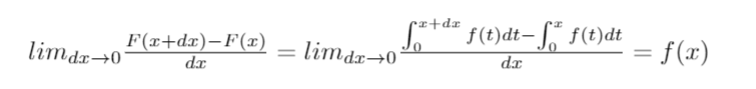
Where, in the second line, we have just plugged in our definition of F(x) as the area under the curve, using the notation introduced above.

Part IIIa: A Proof using Algebra

We now prove

First we observe that

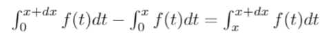
This is because we are only interested in the area between x and x+dx. This is seen in the diagram below, where we are really interested in the red area.

So, the problem then is to work out what the following limit is:

Here we assume the f(t) is continuous at t = x. (We can actually use a weaker assumption, but it requires more effort, as we will see in the final section)

What is the definition of continuity at x? This will take a bit of time to wrap your head around! (Read through the definition twice, then continue, as I will explain it in more informal language)

What does this mean? It means for any (small) number, we can find a small band around x where f(t) is less than that small number away from f(x). For instance, you might set the ‘small’ number to be 0.001. Then, I might find that if t is less than 0.00001 away from x, then we are guaranteed that|f(t) — f(x)| < 0.001. In this case, suppose x = 8, then |f(8) — f(8.000001)|<0.001, because 8.000001 is less than 0.00001 away from 8 (count the zeros!).

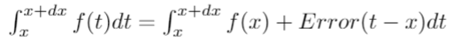
The idea is that as our input t gets ‘arbitrarily close’ to x then f(t) gets arbitrarily close to f(x). One way of representing this idea is to write:

Basically, we write f(t) as the sum of two parts: f(x), and how much f(t) is different from f(x), which is the ‘Error’ term of our approximation. The Error term of our approximation tends to 0 and t gets close to x.

In other words the maximum error within a strip containing x tends to 0 as the strip’s length tends to 0. I made the following diagram to illustrate this:

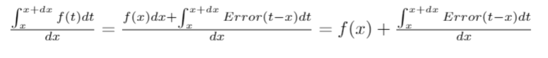
We use this to re-write the equation:

However, f(x) is just a ‘constant’ term with respect to dt.

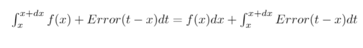
Going back to the diagram from previously, the red rectangle represents f(x)*dx, and the blue shaded area represents the integral of the error terms.

We are quite close to being finished!

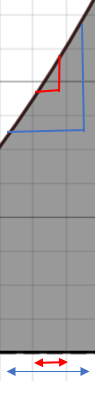
All we want to do is show that the integral of the error, divided by dx, tends to 0. Recall the definition of continuity. If we set our closeness target at 0.01, then for all t suitably close to x, the error term is within 0.01. Then, we would be integrating something of width dx, and maximum height 0.01. So the value of the integral divided by dx would be at most 0.01*dx/dx = 0.01.

A visual demonstration is below: the green arrow double sided arrow represents the maximum error term within a ‘dx’ distance from x. Clearly, the area of the purple rectangle is an overestimate of the error, as its height is always greater than or equal to the maximum error. The diagram shows that the height of the purple rectangle is the maximum error, and the width is dx.

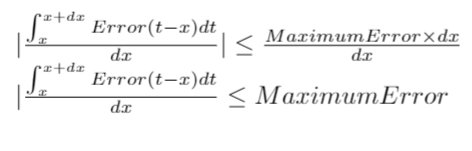
So, provided Maximum Error tends to 0, the integral of the error divided by dx tends to 0 also!

But, as we have already seen, the maximum error within an increasingly narrow strip does tend to 0.

Thus we conclude that:

Part IIIb: A more general proof, and a more rigorous approach?

It turns out our approach can still be improved. For starters, how should we define the integral? ‘Area under a graph’ is useful as a concept, but it isn’t going to help us if we want to use these ideas from calculus on functions and situations which don’t have nice graphs.

However, I am not going to flesh out every detail of what is the culmination of an introductory Analysis course, just give a broad overview.

Lower Partition Sum

A lower partition is an underestimate of what we want the integral to be.

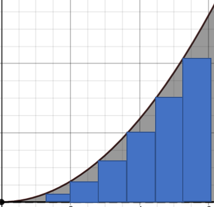
We draw rectangles underneath the graph, and sum up their area. As the rectangles are lower than the graph at every point, this provides an underestimate of the area.

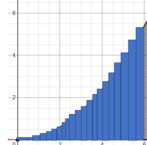
As we make the base of the rectangles thinner, we get and better and better approximation

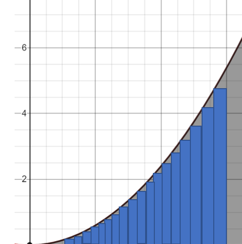
Upper Partitions Sum

This is like a lower partition, but we overestimate the function

Till Death Does Us Part(ition) — using partitions to define the Riemann Integral

To define the integral, we then look at the limit of the values of Lower Partition Sums and Upper Partition Sums as the width of the rectangles’ base tends to 0. If these two values are the same, we say that the Riemann Integral exists.

To then prove the Fundamental Theorem of Calculus, we have two options. If we assume that f(x) is continuous, we proceed as above. If we merely assume f(x) is Riemann Integrable but not necessarily continuous, we have to fiddle around with the lower and upper sums and use some other tricks.

Epilogue: Cracking Previously Impossible Problems

All in all, in hindsight, the theorem was hard to prove, but now it cracks open some really really hard problems. As is so often the case in mathematics, the most important theorems find the most relevant information about a whole class of problems, and then enable mortals (like me and you) to solve problems which even geniuses struggled to solve previously. In fact, this is a lot of the value of a mathematics degree! Let’s crack such a problem open now.

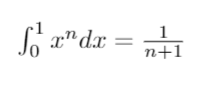
To solve this, we just spot that x^(n+1)/(n+1) differentiates to x^n using the rules for differentiating a polynomial (you can prove this using the binomial expansion if you are feeling keen). Then, by the Fundamental Theorem of Calculus, F(x) = x^(n+1) /(n+1) gives the formula for the area between 0 and x. Plugging in x = 1 gets the answer.

Could you do this without the Fundamental Theorem of Calculus?

The Role of Intuition and Visual Thinking in Mathematics?

What’s interesting about the Fundamental Theorem of Calculus is that without human intuition and visual thinking it would have been near impossible to come up with the relevant definitions in the first place. In fact, in the rigorous partition definition seen in Part IIIb, we started off with an idea of what we thought the area should be and then crafted a definition which we thought would recover that idea.

But it then required our ability to make language precise to turn these thoughts into mathematical objects which can be manipulated in different contexts, for instance using integration with many variables, or even infinite variables, and eventually generalising to Lebesgue’s theory of integration, or integration on weird and wonderful surfaces using differential geometry.

Resources for learning more

For derivatives: An interactive tool by geogebra can be found here if you want to play around a bit. If you have a bit more time and are unfamiliar with derivatives, then this 3Blue1Brown video gives a really nice geometric view on derivatives of certain functions which gives a different way of visualising them.

For calculus: 3Blue1Brown’s Essence of Calculus series is nice. Tom Korner’s Calculus for the Ambitious is a good read. Khan Academy also has very helpful introductory calculus resources.

P.S.

I welcome all feedback, good and bad (but hopefully constructive). If you have a recommendation on how I can make the proof easier to understand and I think the suggestion is a good one, I will try to act on it — Ethan