In physics, events characterized by a significant difference in size (for example, the behavior of waves in the oceans and of their individual water molecules) have a small influence on one another (they do not communicate). Therefore we can independently study the physical properties corresponding to each order of magnitude. This scale independence is precisely what allows us to use hydrodynamics to model ocean waves, ignoring the behavior of individual water molecules. In other words, theories are only successful because physics at different scales can be modeled using different theoretical frameworks (see Wilson).

However, there exists a class of phenomena called critical phenomena where events of different scales make contributions with the same importance (see Wilson for more details). The example given by Wilson is the liquid-vapor critical point.

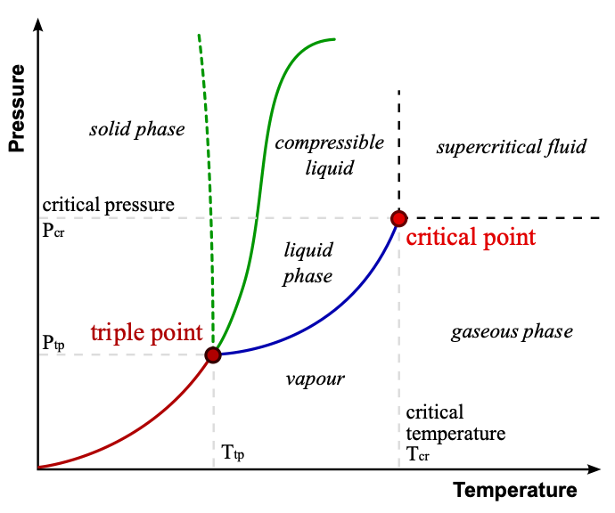
Close to the liquid-vapor critical point, the physical properties of both phases become increasingly similar. At the critical point, they become “a single, undifferentiated fluid phase.” The liquid exhibits density fluctuations “at all possible scales.” Quoting Wilson:

“The fluctuations take the form of drops of liquid thoroughly interspersed with bubbles of gas, and there are both drops and bubbles of all sizes from single molecules up to the volume of the specimen. Precisely at the critical point the scale of the largest fluctuations becomes infinite, but the smaller fluctuations are in no way diminished. Any theory that describes water near its critical point must take into account the entire spectrum of length scales.” — Kenneth Wilson (1979)

Another Example of Critical Behavior

A ferromagnet is a magnetic material where domains are formed (see figure below). In these domains, the magnetic fields of the individual atoms align. However, the orientation of the magnetic fields of each of the domains is random. The net magnetic field is, therefore, zero. However, when an external magnetic field is applied, the magnetic fields of all domains line up in the direction of this applied field, which causes the external magnetic field to be intensified.

Another way for a ferromagnet to exhibit an external macroscopic magnetic field is to reduce its temperature. Below some critical temperature, rotational invariance is spontaneously broken, and a macroscopic magnetic field (in some previously unknown direction) is exhibited even in the absence of an applied external magnetic field.

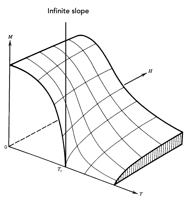
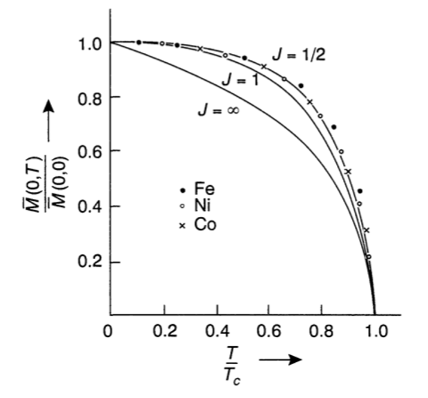
Here, the magnetization M is equal to the average magnetic moment of all atoms inside a region much larger than the typical scale where the relevant microscopic physical processes occur:

When the temperature is increased above this critical temperature the macroscopic magnetization disappears. This transition is in fact extremely sharp. As |M| approaches the value|M|=0, the function |M(T)| has an infinite slope. This (singular) behavior is an example of a critical phenomenon.

Ferromagnetism is a consequence of the so-called exchange interaction between electron spins acting together with the Coulomb repulsion.

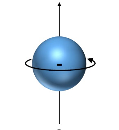
Let me first clarify two concepts. First, what is the meaning of spin? Loosely speaking, spin is “an intrinsic form of angular momentum carried by elementary particles, composite particles, and atomic nuclei.” Though spin is by definitiona quantum mechanical object (there is no concept of spin is classical physics) people often depict particles with spin as small tops rotating around their own axis.

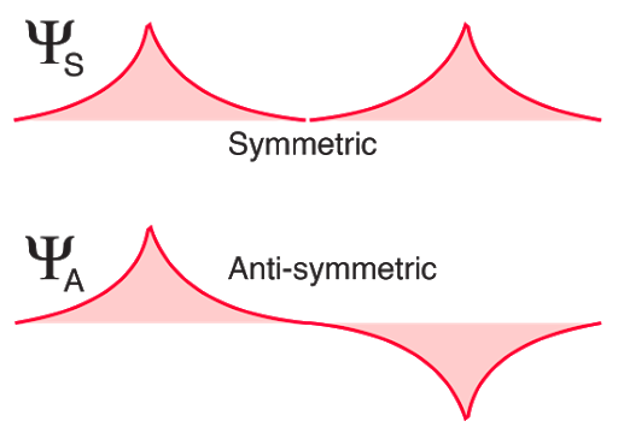
Second, what are exchange interactions? They are quantum mechanical effects that occur between identical particles such as electrons. These effects are a consequence of the fact that the wave function of identical particles is subject to exchange symmetry “either remaining unchanged (symmetric) or changing sign (antisymmetric) when two particles are exchanged.”

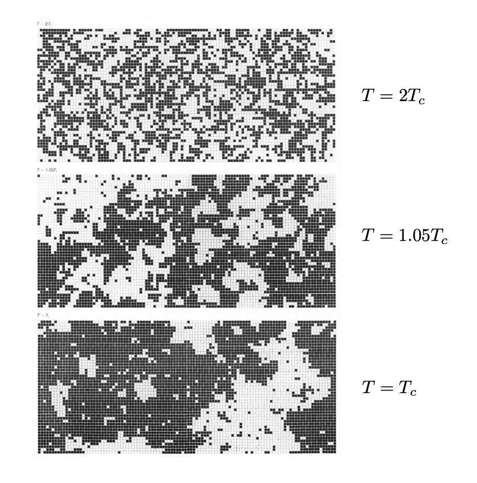
As in the water-vapor critical point, several length scales are involved at the critical point. This is shown in the figure below, which describes some hypothetical solid. Each of the squares corresponds to the orientation of a spin (more specifically, to the corresponding magnetic moment) of a single atom in the solid.

Following Wilson we choose:

• Black squares to represent “up” spins
• White squares to represent “down” spins

The top figure shows the solid above the critical temperature. There, the system is disordered (more, specifically, the order of the spin patterns formed is short-ranged). In the middle figure, when the temperature is lowered, more extensive patches start to appear. The third figure shows the system at the critical point (called Curie temperature). We see that the patches “expand to infinite” scales, but fluctuations at smaller scales continue to exist. Consequently, in this case, one must include all length scales to build a theoretical model of the ferromagnet.

Why Study Critical Phenomena?

Critical phenomena are particularly fascinating mainly because of three reasons (see Stanley):

• Physicists do not fully understand the underlying microscopic phenomena
• Different physical systems exhibit a remarkably similar behavior close to the critical point. A well-known example is the similarity between a ferromagnet and a simple fluid when each is near its critical point. In fact, the numerical values of the critical-point exponents are equal for several groups of seemingly distinct systems.
• According to Stanley, the third reason is awe. He remarks: “We wonder how it is that spins ‘know’ to align so suddenly as [we approach the critical temperature]. How can the spins propagate their correlations so extensively throughout the entire system?

The Partition Function

To study the properties of a ferromagnet in thermal equilibrium at some temperature T, for example, we should in principle write down its partition function. A partition function Z of a system describes its statistical properties when it is in (thermodynamic) equilibrium and it is written in terms of the Hamiltonian H of the system. Most of the thermodynamic variables of a system, including its total and free energies, entropy, pressure, magnetization, and so on, can be written in terms of the partition function (or its derivatives).

The partition function is given by:

where H is the microscopic Hamiltonian. We can also write Z as:

where G is the Gibbs free energy. The latter is important because it helps to identify the equilibrium state of a system. This occurs because if we keep the system at constant temperature and pressure, the Gibbs potential is minimized when the system is at equilibrium.

For nonzero temperature, Z seems to be a smooth function of T with the exception of the non-analytic (of M(T)) behavior at the critical temperature.

Ginzburg–Landau theory

However, in most cases of complex systems, Z cannot be calculated and therefore one cannot start the analysis using the microscopic Hamiltonian.

The two renowned Soviet physicists Lev Landau and Vitaly Ginzburg reasoned that another way to write the free energy G (of a system of volume V) in terms of the magnetization M would be to take into consideration symmetry properties of G with respect to M. The magnetization (or any other quantity that becomes nonzero after such a transition) is usually called an order parameter.

The mathematical form of this vanishing of M just below the critical temperature is known experimentally to be:

For example, if M is constant in x, rotational invariance would restrict the free energy G to:

The prefactors a,b,… are unknown but we suppose they are smooth, well-behaved functions of the temperature T (no singularities or discontinuities). Supposing, following Landau and Ginzburg, that a vanishes at some critical temperature it is natural to conjecture that close to this temperature,

A Quick Interlude: Breaking a Continuous Symmetry

How to calculate the minimum of a functional such as G(M)? Consider Tue case where M has two dimensions:

The minimum occurs at, for example:

where the second component can be equal to any value situated in the circular base of the potential shown below (M₂=0 is just a convenient choice):

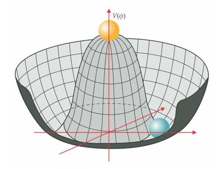
At temperatures above the critical temperature, the minimum of G occurs at M=0 but for temperatures below the critical temperature there are new minima (derived above):

We see that rotational symmetry is spontaneously broken and a non-analyticity appears. This is an example of a second-order phase transition, a type of critical phenomenon.

Now, this G is too simple and we must include spatial variations of M. Landau and Ginzburg suggested the following generalization:

where we can rescale M to make the coefficient of the first term equal to 1.

In the presence of an external magnetic field and above the critical temperature, G becomes:

When H ≠0, the non-analyticity disappears, and |M| becomes a regular function of the temperature.

For small M, minimizing G gives us the following differential equation:

which has the following solution:

Integrating over k we obtain:

Now consider a magnetic field H localized at x=0 which generates a magnetization M(0) at the origin. What is the magnetization M(x) for x ≠ 0?

Here the concept of the correlation function is important. The correlation function measures the order in a system, how microscopic variables at different positions relate to each other, and how they co-vary with one another on average (across space and time). In our case it is:

What is the behavior of C(x), or equivalently of M(x), for large |x|? In other words, how do these quantities decay?

The decay is given by:

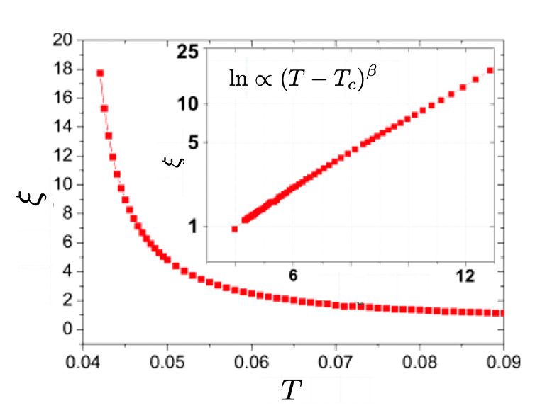
This indicates that there is a correlation length ξ over which the correlation function decays and that this length diverges (goes to infinity) as T approaches the critical temperature.

Performing this calculation using the Landau-Ginzburg theory we find:

Using Eq. 14, we find that the value of the exponent ν is 1/2.

Critical Exponents, Scaling, and Universality

Critical exponents such as ν and β define the nature of singularities at the critical point for many physical quantities, including heat capacity, susceptibility, and so on.

But why are critical exponents so important? It turns out combinations of these exponents give origin to laws of scaling which are a type of universality. It has been found experimentally that some radically different systems with completely different critical temperatures have the same scaling exponents where the latter are combinations of critical exponents.

For example, using the critical exponents we found above we obtain the so-called Fisher scaling:

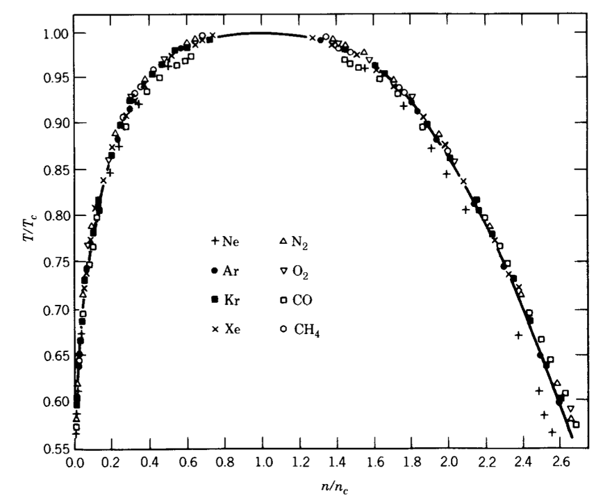
Another example is shown in Fig. 12 for the gas-liquid coexistence region.

The relation between exponents is one of two manifestations of the so-called scaling hypothesis. The second one is called by Stanley, “data collapse”. Following Stanley, consider a uniaxial ferromagnet. The magnetization M depends on H and on the reduce temperature ϵ:

Plotting M/H to some power vs. ϵ/H to some other power there is a collapse of the data into one curve. For example, the relation between these two quantities for five different substances (see Stanley) gives us the plot below:

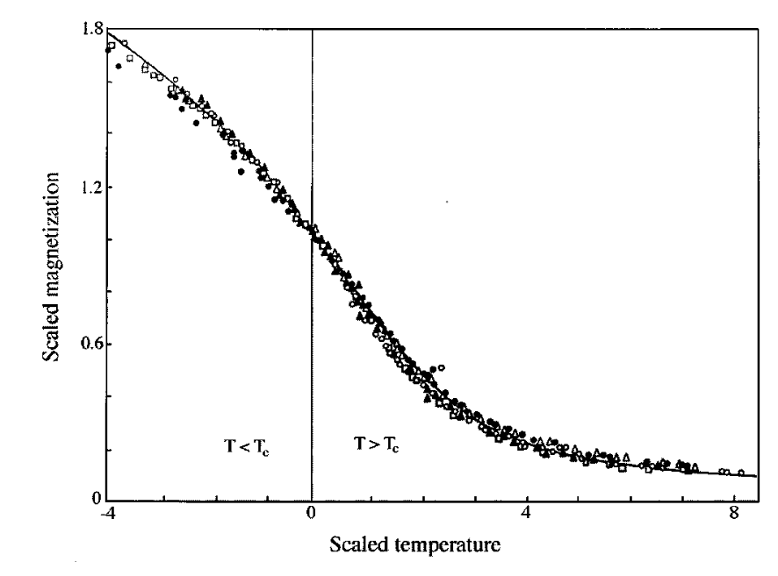
Another fascinating property found at criticality is universality. Fig. 13 above shows an example: since all five materials have the same exponents and scaling functions they belong to the same universality class. Critical systems can be divided into such classes, similarly, as noted by Stanley, to a mind of Mendeleev table.

A more complete theory of critical phenomena can be obtained using the concept of the renormalization group. However, to explain this concept a whole new article would be needed. You can have a preliminary notion from one of my previous articles, linked below.

Deep Learning Explainability: Hints from PhysicsDeep Neural Networks from a Physics Viewpointtowardsdatascience.com

Thanks for reading and see you soon! As always, constructive criticism and feedback are always welcome!

My Linkedin, personal website www.marcotavora.me, and Github have some other interesting content about physics and other topics such as mathematics, machine learning, deep learning, finance, and much more! Check them out!