
The Coupon Collector Problem
We discuss the well-known Coupon Collector problem, and provide two ways of computing the probability of winning.


Suppose your favorite brand of cereals is having a competition, where in each box of cereals there is a coupon with a positive integer number between 1 and N, and you win a prize if you collect coupons with all numbers between 1 and N. Moreover, when you buy a new box of cereals, the coupon inside the box independently from other boxes has the number i with probability 1/N, for every i = 1, …, N.
The obvious question to ask now is the following.
How many boxes do we need to buy in order to have good enough probability of winning?
The above problem is very well studied, and is usually called the “Coupon Collector problem”. In this article, we will give some ideas about how one can approach it.
What is the expected number of boxes we need to buy in order to win?
Since we are dealing with randomness, a natural first question to ask is about the expected number of boxes one needs to buy in order to win.
To compute this expectation, for every i = 1, …, N, we define the random variable Xᵢ as follows. X₁ is equal to the number of boxes we need to buy until we have one distinct coupon in our collection. Clearly, we always have X₁ = 1, since we start with zero coupons in our collection. We continue with X₂, which is equal to the number of additional boxes we need to buy (not counting the X₁ boxes we have already bought) until we have two distinct coupons in our collection. Similarly, X₃ is the number of additional boxes we need to buy (not counting the X₁+X₂boxes we have already bought) until we have three distinct coupons in our collection, and so on.
Let’s clarify this a bit with an example. Suppose N = 3, and here is a sequence of boxes with their coupons that we end up buying, one by one, from left to right:
1, 1, 3, 1, 3, 3, 2.
In the above example, we have X₁ = 1, since we always discover a new coupon in our first box. Then, the second box contains a coupon with the number 1, which we already have. We continue and buy the third box, which now has a coupon with the number 3. Thus, X₂ = 2, since we had to buy two additional boxes in order to discover a new coupon. We continue and we see that we have to buy four additional boxes in order to discover a new coupon, namely a coupon with the number 2. Thus, X₃ = 4. In total, we ending up buying X₁+X₂+X₃ = 7 boxes in order to discover all numbers and win. We conclude that, given the above definition of random variables, the total number of boxes we need to buy in order to win is

So, the goal now is to compute the expected value of the random variable X, which describes the sum of the random variables Xᵢ, for i = 1, …, N. To do so, we will use an extremely useful property of the expected value, which is called Linearity of Expectation. This implies that

Thus, the main task now is to compute E[X]ᵢ, for i = 1, …, N. We start with X₁. As we discussed, we always have X₁ = 1, and so we get that E[X₁] = 1.
We continue with X₂. Since we have already collected one coupon (it does not matter which number it has on it), the probability of collecting a coupon with a new number if we buy one new box is (N-1)/N. This is because the only way that we are not getting a new number is when the new box contains the same number as the one we already have in our collection. Since we only have one number, the probability of ending up with the same number in the new box is exactly 1/N, and so the probability that we get a new number is 1–1/N = (N-1)/N. In other words, if we focus only on one new box, the probability of “success” is (N-1)/N. By assumption, each new box independently contains a number i with probability 1/N. This means that the random variable X₂ has a geometric distributionwith probability of success (N-1)/N. We will not go into details about the geometric distribution; the interested reader can look here for more information. The only property we need from the geometric distribution is that its expected value is 1/“probability of success”, and so we conclude that

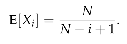
Continuing in a similar way, for the variable Xᵢ, the probability of success when we buy a new box is exactly equal to 1-(i-1)/N= (N-i+1)/N, since we already have i-1 distinct coupons in our collection. Thus, its expected value is
Putting everything together, we get that
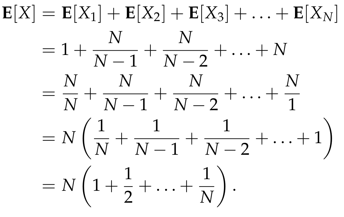
The term in the parenthesis in the above expression is the well-known N-th harmonic number, which for all practical purposes, is almost equal to ln N (if you want to learn a bit more about the harmonic numbers, you can have a look at another post of mine on the subject). Thus, we conclude that
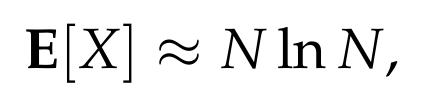
or if we want to be slightly more careful and get a bound that always is correct, we get that

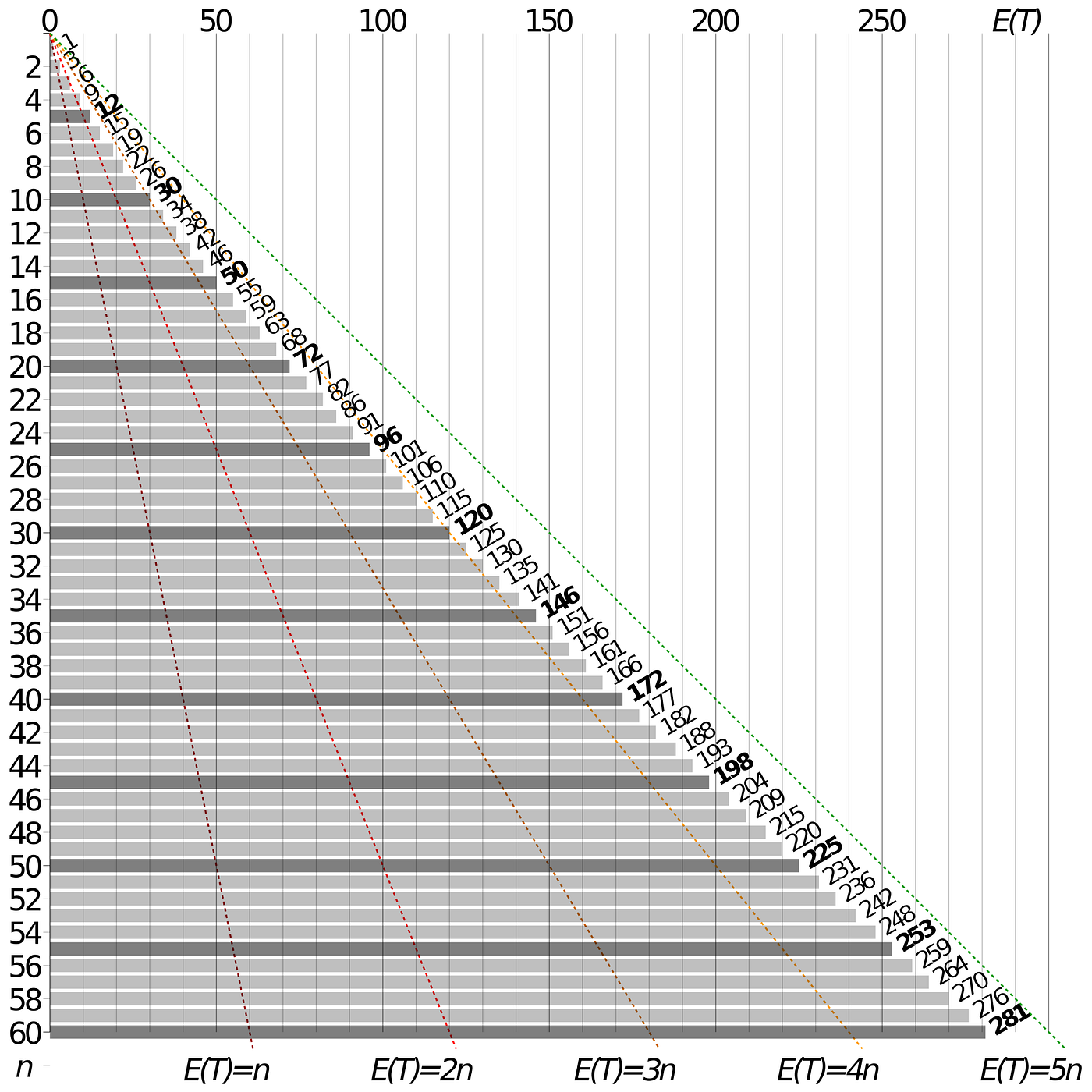
To get a sense about the value of E[X] for various values of N, here is a graph.
The above discussion shows that we can actually compute the expected number of boxes we need to buy in order to win. But, often, the expected value does not reveal too much, especially in cases where it has very large variance. So, we will now discuss a bit more about the probability of needing to buy many more boxes than what the expected value suggests.
What is the probability that we end up buying more boxes than what the expected value tells us?
A first and very straightforward approach for that is to use Markov’s inequality, which states that if X is a non-negative random variable, then for any number t > 1, we have
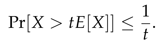
If we plug in t = 2, then we get that with probability at least 50%, we will not need to buy more than 2E[X] ≤ 4N ln N boxes.
Similarly, with probability at least 75% we will not need to buy more than 4E[X] ≤ 8N ln N boxes.
[For more information about Markov’s inequality, you can check Wikipedia, or the multiple sources available online, or a previous article of mine on the topic.]
These bounds are already good enough, but we can actually get much stronger results with a slightly more careful analysis.
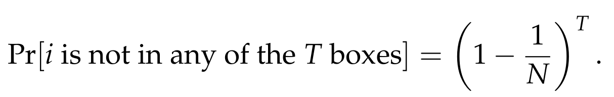
For that, suppose that we decide to buy T ≥ 1 boxes. We now compute the probability of not getting a coupon with the number i in any of these T boxes. As already explained, the probability that we do not get the number i in single box is 1–1/N. Since each box is independent from the others, we get that the probability of not getting the number i in any of the T boxes is
We now use the following very useful inequality, that holds for every real number x:
Plugging in x = -1/N, we get that

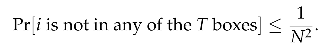
We now set T = 2N ln N, where we round up to the next integer, if 2N ln N is not an integer. Thus, we get the following:
We are almost done. Since we have N distinct coupons, we now apply the very useful Union Bound, which can always be applied, regardless of whether the events in question are independent or not. Formally, we consider the N events, where each event corresponds to the event of the number i not being in any of the T boxes, for every i = 1, …, N. We conclude that

In other words, if we buy T = 2N ln N boxes, then the probability of winning is at least
The above bound gives a much stronger concentration bound as N grows, compared to Markov’s inequality, and suggests that we almost surely win if N is large enough and we decide to buy T = 2N ln N boxes!


