The invention of group testing dates back to WWII, as the U.S. army wanted to weed out all syphilitic men called up for enlistment. The presence of syphilis could be identified with a blood test. However, individually testing the blood sample of each new recruit costed lots of time and resources. Thus, the U.S. army had to face the following problem:

Is it possible to test N people with less than N tests?

The statistician Robert Dorfman had a brilliant idea to minimize the number of blood tests required. He proposed that:

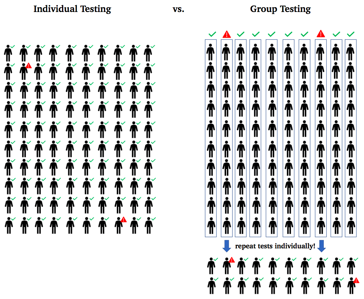
The blood samples of k people can be pooled and analyzed together. If the test is negative, this one test suffices for the group of k people. Instead, if the test is positive, each of the k persons must be tested again separately, and in total k+1 tests are required for the group of k people.

The principle of group testing is summarized in the figure below.

What’s the performance of group testing? Dorfman showed that it depends on the probability p that a recruit is infected and, importantly, on the choice of the group size k.

Here, we will reproduce Dorfman’s computations in order to evaluate the performance of group testing. The following steps are needed:

1. Compute the group-outcome probabilities
2. Calculate the total number of tests required
3. Optimize the group size k, for a given prevalence rate p

Note: the practical effectiveness of group testing depends also on the sensitivity of the test, which is specific for the considered illness. In the following, we will assume that test outcomes are always reliable.

1. Group Probabilities

Let p denote the probability that a single person is infected. This corresponds to the prevalence rate of the considered disease in the population (it was syphilis for Dofrman’s analysis, or Covid today…). Thus, p is the independent variable of the problem and is assumed to be known. It is convenient to define q=1-p as the probability that a person is healthy.

The pooled test for a group of k people will be negative if all of them are healthy. We find the probability P(-) of this event as:

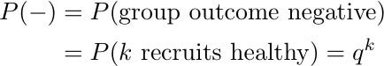
Conversely, the test outcome of the group is positive if at least one person is infected. The probability P(+) of this scenario is complementary to P(-):

We can think of the test outcome of each group as a coin toss, which decides whether the group is healthy or needs to undergo the individual test round. More precisely, we can say that the outcome is a Bernoulli random variable with “success probability” equal to P(+).

2. Expected Number of Tests

Given a total of N recruits, we can now compute the number of tests required within the group strategy. This number is random, since it is subject to the probabilistic outcomes of all groups (see footnote¹). Nevertheless, we can study its expected value.

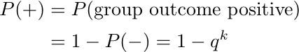
First of all, each of the N/k groups receives one initial test. Next, whenever a group gets a positive outcome, k additional tests have to be performed. Overall, the expected number of tests, E[T], reads

We see that the result is proportional to N, the total number of recruits. Thus, the term f(k,p) can be interpreted as the expected number of tests per person: the initial test counts as 1/k because is shared with the group, and then an individual test occurs with probability P(+).

Whenever f(k,p) is less than 1, group testing is more efficient than performing Nindividual tests. The following plot illustrates that, for each prevalence rate p, there is a group size k* for which the number of tests is minimized.

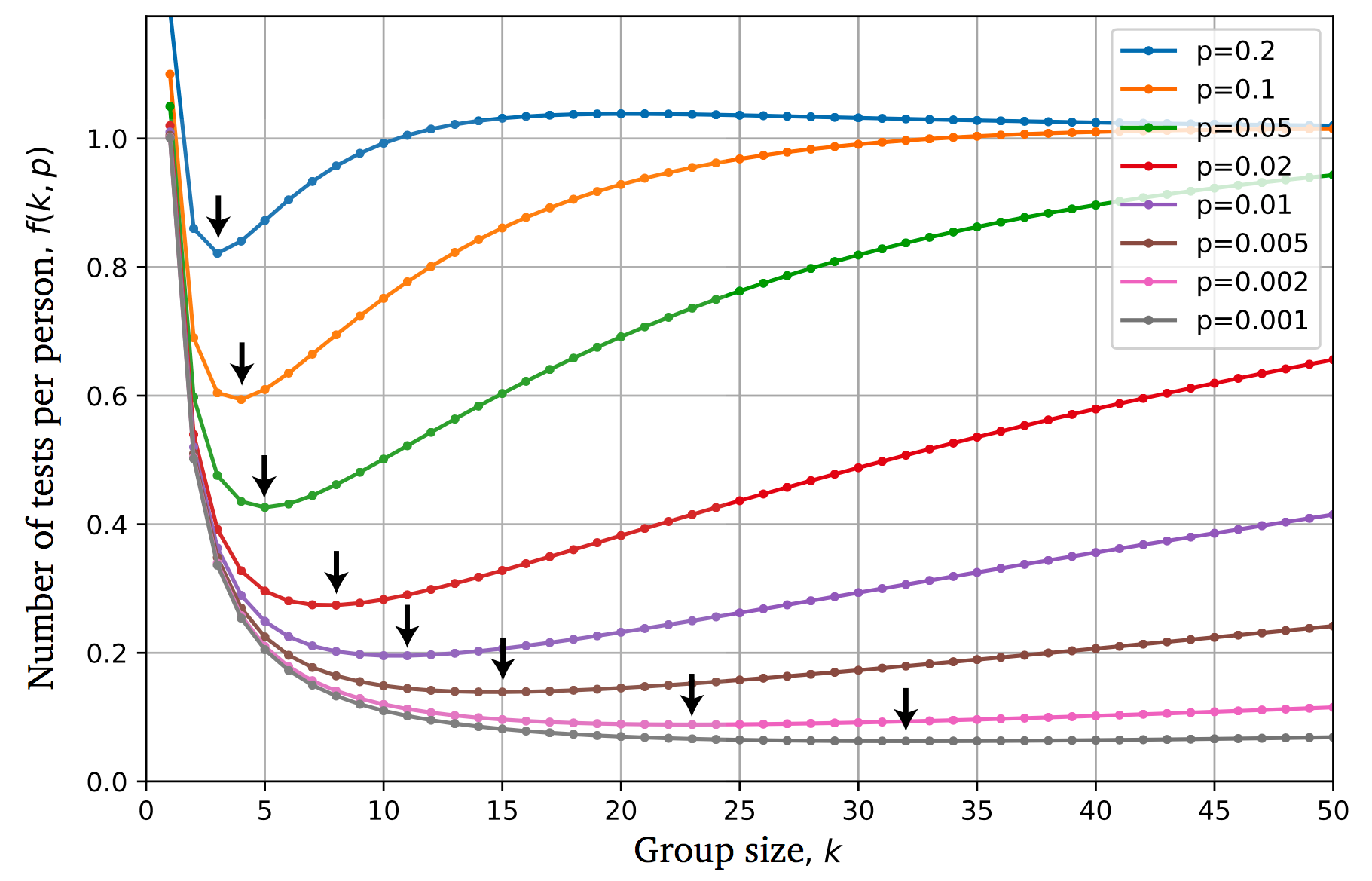
By following the trend of the arrows in the plot, we can appreciate that

the rarer the prevalence of the disease, the larger the optimal group size gets.

This makes sense because, with lower p, it will be more likely that larger groups will get a negative result: so, we can save on tests by pooling more people together.

Next, our goal is to derive a formula to determine the optimal group size k*.

3. Optimal Group Size

For a given prevalence rate p, the optimal group size k* is found by minimizing f(k,p), the expected number of tests per person. Therefore, we set the partial derivative of f(k,p) with respect to k equal to zero:

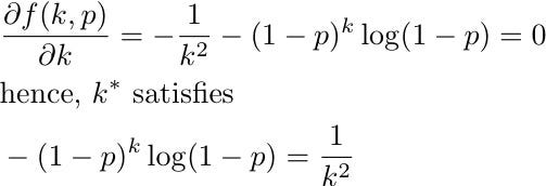
Unfortunately, this equation does not admit an explicit solution. However, since the value of p is typically small, we can proceed with a Taylor expansion around p=0 as follows

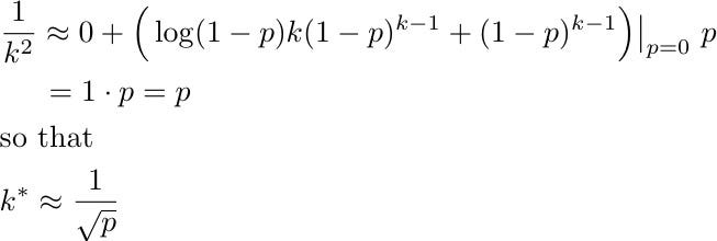
The obtained approximation is of great practicality. For small p,

the optimal group size k* is well approximated by the inverse of the square root of p.

For instance, we find k*=5 for prevalence rate 5%, k*=10 for p=1%, and k*=32 for p=0.1%.

4. Employing Optimal Group Testing

We can explicitly check how many tests E[T*] are required on average with the optimal group size by substituting the approximated formula for k* into E[T]. By Taylor expanding again for small p, we get:

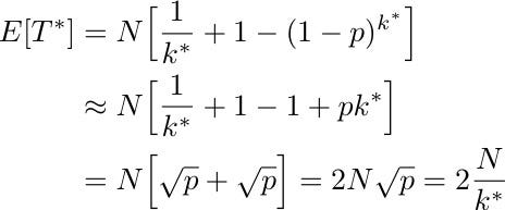
Whenever p<1/4, we see that E[T*]<N and, therefore, group testing is more efficient than individual testing (²). Since 1/4 is a remarkably high prevalence rate, this basically implies that group testing is a better solution in most of the practical situations.

We can appreciate that the efficiency of group testing is higher and higher the smaller the prevalence rate p is. For instance, considering N=1000recruits, the expected number of tests would be

• E[T*]=400 for prevalence rate p=5% and k*=5.
• E[T*]=200 with p=1% and k*=10.
• E[T*]=63 for p=0.1% and k*=32.

All of these cases achieve a much lower number than N=1000 individual tests. Group testing is smart.

We can plot the approximated optimal number of tests per person f(k*(p))=E[T*]/N=2/k* and appreciate how it passes through the minima of the curves f(k,p).

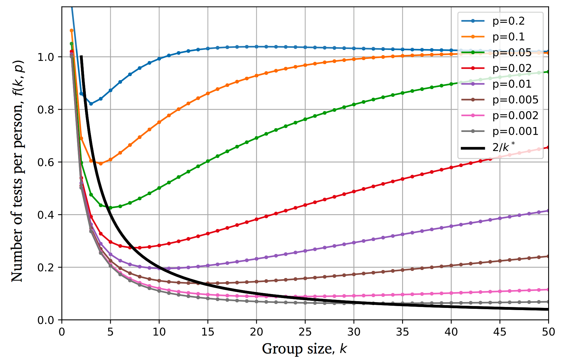
Note that f(k*(p)) can be also interpreted as the overall relative testing cost of the group strategy. For example, for p=1% we can save 80% of the tests.

Summarizing, we found that:

1) Group testing is incredibly more efficient than individual testing, especially with small prevalence rate p.

2) The expected number of tests is approximately 2N/k*, with optimal group size k* given by the inverse of the square root of p .

Dorfman’s Legacy: Group Testing

Robert Dorfman published the blood-testing strategy against syphilis in a short research article in 1943, as he was serving as an operational analyst in the U.S. Army Air Forces. His contribution not only saved millions of lab analyses, but also set the start of the field of applied mathematics named group testing.

Group testing is an object of research still today and has found several applications across different fields of science and engineering.

Footnotes

(¹) Technically, the number of groups to be retested follows a Binomial distribution with number parameter N/k and success probability P(+) as defined above. A Binomial random variable simply describes the amount of positive outcomes out of a given number of independent coin tosses. The expected value of a Binomial random variable turns out to be the number of coins (here, of groups) times the probability P(+) of positive outcome.

(²) Please, note that all results obtained after a Taylor expansion are approximated, although accurate for small prevalence rate p. Some of the values reported above might be slightly different if obtained with an exact numerical optimization.