The Best Numerical Derivative Approximation Formulas

Approximating derivatives is a very important part of any numerical simulation. When it is no longer possible to analytically obtain a value for the derivative, for example when trying to simulate a complicated ODE. It is of much importance though, as getting it wrong can have detrimental effects on the solution. In this article, I will demonstrate the finite difference approximation schemes and show their accuracy.

Let me start with the standard definition of the derivative:

1. Forward difference

Taking the limit of the above function as hgoes to 0 is numerically infeasible (a computer can’t do it), so the first thing that comes to mind is to take a small h , and calculate the value of the derivative. This is called the forward difference scheme.

2. Backward difference

The backward difference scheme is an alternative method to the forward difference scheme, where instead of adding h , we can subtract h from x, to get. It has some advantages, for example, when trying to estimate the derivative of a function at the same time as we calculate the function itself. It is also a more stable method, even though it has the same accuracy as the forward difference method. I will discuss accuracy below.

3. Central difference

The central difference estimate is sort of a combination of the above two. We subtract the function value immediately below f(x) from the function value immediately above f(x). It is the most stable and has an order higher accuracy.

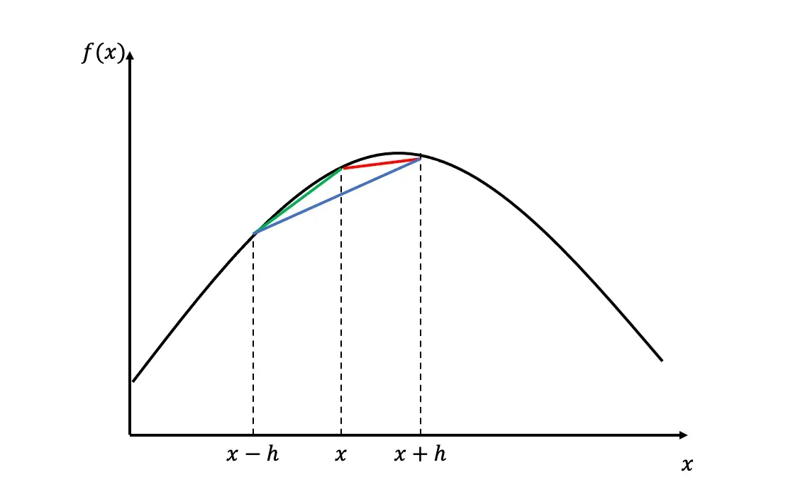
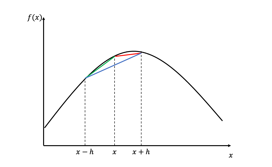
The forward, the backward and the central difference scheme are often referred to as the finite difference schemes. The picture below illustrates how they differ from each other. Note, that to calculate the central difference scheme, we don’t need to know the value of the function at x .

Code

One can easily implement these in python by writing functions for them. To demonstrate it I will be using the function f(x)= -(x-5)^2 + 100 . The coded functions will take input f(x) and x and will return the slope of the tangent line.

import numpy as np
import matplotlib.pyplot as pltdef f(x):
return -(x-5)**2+100def forward_difference(f,x0,h):
d = (f(x0+h) - f(x0))/h
return ddef backward_difference(f,x0,h):
d = (f(x0) - f(x0-h))/h
return ddef central_difference(f,x0,h):
d = (f(x0+h) - f(x0-h))/(2*h)
return d

With the finite-difference schemes implemented, we can now test the accuracy of the methods. We know that the derivative of f(x) at x=10 is f'(x=10) = 10 by analytically differentiating the function and plugging in.

Accuracy

To test the accuracy of the finite difference methods, I will look at the difference between the estimates and the true value as I decrease h .

error_fd = []
error_bd = []
error_cd = []h = 0.1
for i in range(1,30):
fd = forward_difference(f,10,h/i)
error_fd.append(np.abs(fd) - 10)

bd = backward_difference(f,10,h/i)
error_bd.append(np.abs(bd) - 10)

cd = central_difference(f,10,h/i)
error_cd.append(np.abs(cd) - 10)plt.figure(figsize=(7,5),dpi=200)
plt.plot(error_fd, label='forward difference')
plt.plot(error_bd, label='backward difference')
plt.plot(error_cd, label='central difference')
plt.xlabel('1 / h')
plt.ylabel('error')
plt.legend()

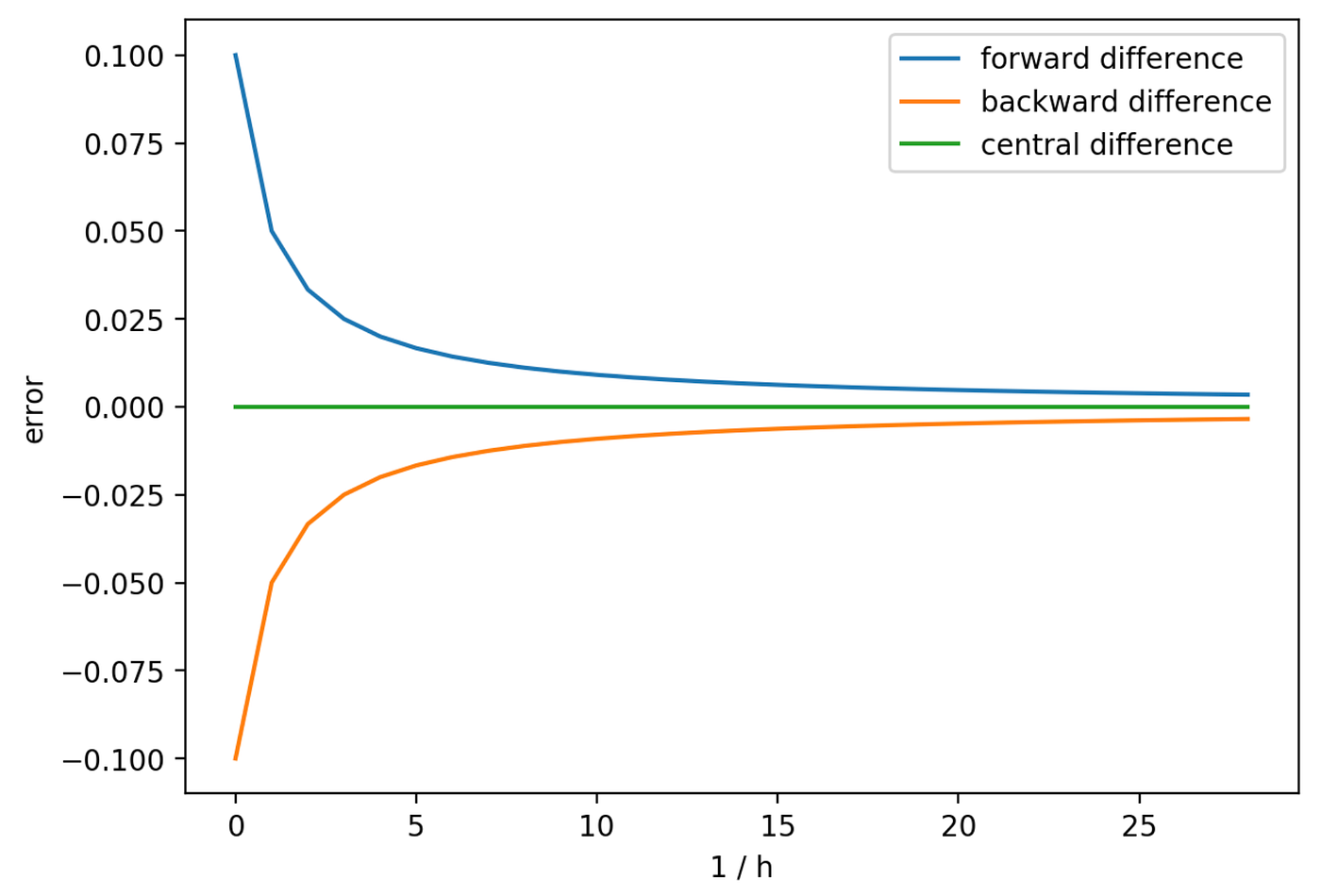
From the above graph, we can see that the forward and backward difference estimates approach the true value of the derivative as we decrease h , from above and from below respectively. The central difference approximation, on the other hand, provides a rather accurate estimate of the true value. As a result, the central difference estimate is usually the most reliable scheme to use.

Proof

Actually, we can prove that the central difference scheme is a more accurate method than the other two. First, let’s see how the accuracy of the forward and backward schemes scale with respect to h. To do this, Taylor expand our at least twice differentiable function around f(x+h) :

For the easy treatment of our problem, keeping only the first-order terms from the Taylor expansion and using the Big-O notation for the rest, we can rearrange the above equation to see that the accuracy is linearly related to h .

C is the supremum for h < h_0 . So, we know that the accuracy of the forward difference is limited by C*h . For the backward difference scheme, we can construct a similar boundary using the same method: Taylor expanding and then rearranging.

Clearly, we can see that they are both of order h accurate. To see the accuracy of the central difference estimate, subtract the two 3rd order Taylor expansions from each other and rearrange.

Subtracting the second from the first, we get

and then dividing with 2h .

C is useful here because it does not change the order of magnitude, it is a multiplier only.

We have now proved that the accuracy of the central difference estimate is of order h^2 , which given that h approaches 0 will be much small than h . As a result, whenever possible it is better to use the central difference estimate that the other two.

Conclusion

In this article, I proved that both numerically and visually that the central difference is more accurate than either the forward or the backward difference estimate. It is important to understand this because when things get more complicated, for example when trying to simulate a PDE, it is crucial not to get the derivative approximations wrong.

It is possible to estimate higher-order derivatives as well with the same methodology and there are some other methods, such as the five point stencil method. To see this applied in practice, have a look at my other articles. I use the finite difference scheme to simulate PDEs.