The Besicovitch 1/2 Conjecture

Here’s a conjecture with a lot of really smart people working on it that has a fairly intuitive statement, and yet almost no one knows about it. Seriously, there isn’t even a Wikipedia page.

The idea is to quantify how weird 1-dimensional sets can be. We’ll make these notions more precise in a bit, but let’s start with some very basic ideas to make it easier.

Line Segments

If anything is going to be called “1-dimensional” it’s a line segment. If you understand this section, then you’ll have the foundation for the rest of this article.

So, make sure you think through this carefully.

Consider a line segment and a point on the line. We’ll then look at how much of the line goes through a circle centered at the point:

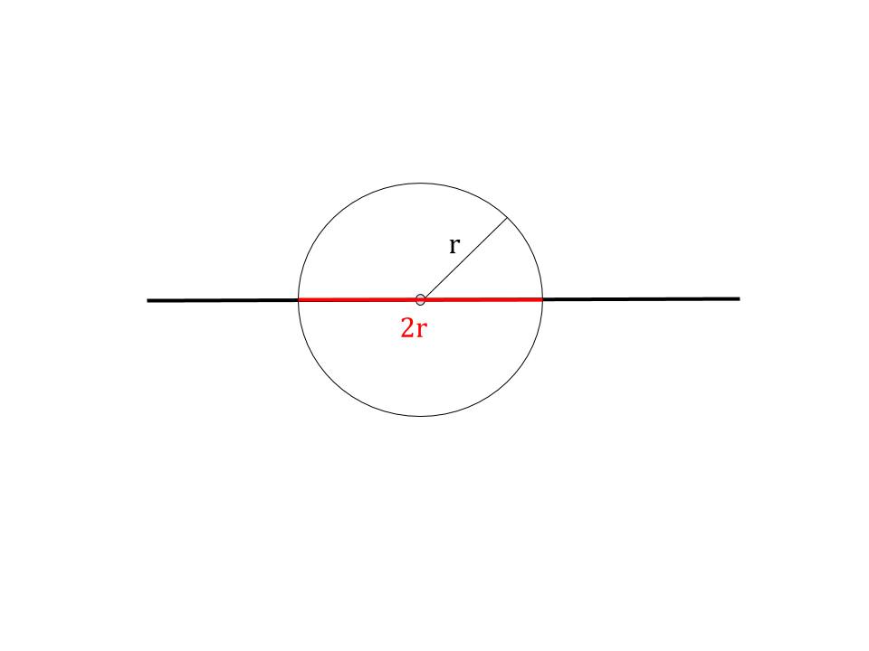
Well, as long as the circle is small enough that it stays on the line, the amount of the line in the circle is 2r.

To measure “weirdness,” we’re only going to care what happens at really small scales (think about how we do this in Calculus with the tangent line). This means we’re going to let r get closer and closer to zero.

Think of this as “zooming in” at the point.

Keeping track of the radius is super important here because it tells us what “scale” we’re at. Again, just think of this like the limit we make in the definition of a derivative.

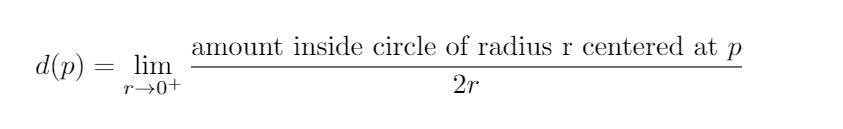
We take the limit of the ratio of the amount of the line segment inside the circle divided by 2r.

As r goes to 0, this ratio will be called the density at p, notated d(p). In the literature, you’ll see this as spherical density, since in higher dimensions we’ll use spheres in place of circles.

Now, this is really easy to compute, because we just said that as long as p is not an endpoint and r is small enough, the amount inside is 2r.

Thus, the ratio is always 1, even without the limit.

Likewise, the endpoint always has r inside, so the ratio is always 1/2.

We’ve now computed the density at every point of the line segment: it’s 1 unless we’re on an endpoint, in which case, it’s 1/2.

Nice Curves

Now we can bump up the complexity very slightly. Let’s consider the types of things we learn about in Calculus: differentiable curves.

There are a few things we could mean by this, but I don’t want to get bogged down in technicalities yet. We’re still developing the intuition.

If you’re being fancy and ready for higher dimensions, you can think of it as the image of [0,1] in ℝⁿ where it makes sense to have a tangent line (no crossing itself, for instance). Alternatively, you could think of it as the graph of a differentiable function in ℝ².

The point is that the curve is 1-dimensional, and except at the endpoints, there is a single tangent line.

Now, I’ve been hinting at this the whole time by making the analogy to the limit in the definition of the derivative.

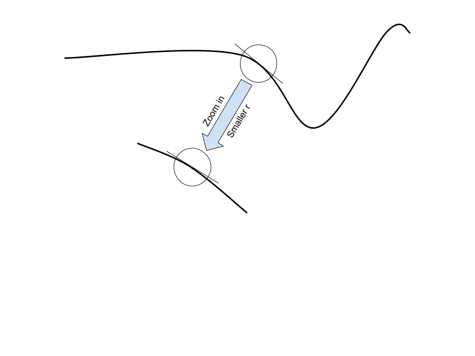
The whole fundamental idea of differential calculus is that when you zoom in at a point, the curve becomes closer and closer to the tangent line.

If you’re familiar with calculus, it might be a good exercise to prove to yourself rigorously that the density at any non-endpoint of a differentiable curve is exactly 1 like the line segment.

And again, we’ll get 1/2 at the two endpoints.

It’s important to note that being differentiable is a really, really strong condition.

But this picture that’s emerging should indicate we’re on the right track for defining some useful measure of “weirdness.” We now know that for nice curves, we get that the density is 1 practically everywhere and then 1/2 at a couple of weird points.

Let this be your intuition going forward because that’s actually pretty close to the precise conjecture.

Large Density and Crossings

Let me burst your bubble for a moment. This isn’t going to be as easy as it seems to this point.

Remember, we’re eventually going to want a conjecture that covers all “one-dimensional sets,” whatever that means.

There are some obvious one-dimensional sets that break from the above scenario that we’ll need to factor in:

This is simply 2 line segments that cross. There is no doubt this should be considered a 1-dimensional set. If we ignore the crossing point, we can always find small enough circles to miss the crossing and we get a density of 1, except at the endpoints, which is 1/2.

But no matter how small we make the circle for the crossing point, there will always be 4r inside. This means the density there is 2.

Now things should be clearer. We can make one-dimensional sets with points that have arbitrarily large density by making it cross itself a bunch like that.

Here’s something that might be fun to think about to develop your intuition even more. Our examples had the density be 1 almost everywhere (don’t worry if you don’t know what that means) and then 1/2 or greater than 1 at isolated points.

• Is this always how it has to be?
• Can you think of something where the density is between 1/2 and 1?
• Can you think of something where the density is greater than 1 or equal to 1/2 for “most” of the set?
• Is less than 1/2 even possible?

Trying to think of what these might look like is helpful for understanding the conjecture, but don’t think too hard because there are theorems that tell us some of that is impossible.

Hopefully that’s some motivation to get through the next section where we have to get a little more technical.

One-Dimensional Sets

We’ll call a set 1-dimensional if it has Hausdorff dimension 1. Actually defining this is beyond the scope of this article, but here’s roughly what to think about.

Hausdorff dimension is usually used when talking about fractals. Fractals can bunch up with jagged edges causing the Hausdorff dimension to be (strictly) between 1 and 2.

For example, the famous Sierpinski triangle fractal has dimension around 1.585.

This means the Hausdorff dimension captures the fact that fractals sort of look 1-dimensional but have extra dimension, too and aren’t quite 2-dimensional.

The point of bringing this up is that specifying the set to have Hausdorff dimension 1 means that it actually has dimension 1 in some real, intuitive sense.

The sets can be really, really weird but not so fractally that we pick up extra dimension.

Here’s an example of a set with dimension 1 that can’t be made in any of the ways we’ve talked about so far. If you’re familiar with characteristic functions, it is the graph of the characteristic function of the rational numbers.

Plot (x,1) when x is a rational number and (x,0) when x is an irrational number.

We tend to visualize this as two lines like the above, but in reality, the bottom piece has holes everywhere and the top piece has practically nothing to it.

Unfortunately, since this is still basically a line, it’s (morally speaking) secretly still of the type we already understand. This is because we can throw out the top piece as irrelevant since it has measure 0.

To put it in the terms above, the density at any point on the top piece is 0 and the density at any point on the bottom piece is 1.

So, this doesn’t help us understand how weird these can be, but I think it helps us understand the type of weirdness a bit better.

It turns out that any one-dimensional set S can be broken down into three distinct pieces: E, R, and U (these aren’t the standard notation).

E stands for empty. It’s the stuff that isn’t actually 1-dimensional.

R stands for rectifiable. It’s the stuff that’s nice like we’ve been talking about. The definition is roughly that it’s almost everywhere pieces of nice curves. Remember that this does include the weird characteristic function above.

The last piece is U for unrectifiable (or purely unrectifiable in the literature). It’s basically defined to be the stuff that’s left over.

Purely Unrectifiable Sets

I think we need to take a moment to think about what 1-dimensional purely unrectifiable sets are before continuing.

Here are two ideas.

• No matter how you zoom in, you’ll get more than one tangent direction.
• It’s like a fractal, but not so much that its dimension is more than 1.

If that’s good enough for you, feel free to jump to the next section.

Here’s an actual construction of one of these things that’s pretty understandable. It’s called the four-corner Cantor set. If you’ve seen the construction of the Cantor set, then this should feel familiar.

Start with a square. Divide it up into a 4x4 grid and remove all but the four corner squares.

Now do that again with those 4 squares.

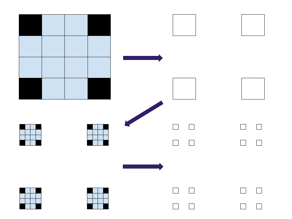
Keep iterating that process, and in the limit, you’ll end up with a set. It’s not obvious this results in something one-dimensional or purely unrectifiable.

But if we keep with our intuition, we should believe it’s purely unrectifiable. First, it’s a process that results in something fractal-like. Second, we’re getting “corners” everywhere which makes the definition of a tangent impossible.

The Besicovitch 1/2 Conjecture

Here’s what you’ve been waiting for.

Take our 1-dimensional set S (in ℝ²) and divide it up into the three pieces E, R, and U.

We throw out the empty bit E as irrelevant.

For our purposes, we’ll say the rectifiable piece, R, is understood. For example, Besicovitch proved in 1928 that for almost all x∈R, d(x)=1. This means that our intuition above was basically right.

The real question is: how weird can the purely unrectifiable piece, U, get?

Remember from Calculus that limits might not exist. Besicovitch proved in 1938 that for almost all x∈U, the limit defining the spherical density does not exist.

If we use a liminf in place of the limit we get what is called the lower spherical density.

Let’s notate that as d_(x). The minus sign represents “lower.”

Here’s a new question: what’s the smallest number, A, such that d_(x) ≤ A for almost every x in U (for any purely unrectifiable U)?

Now, you might be thinking: what on Earth? Why would someone ask that?

Answer: this has a tangible meaning. It’s effectively a numerical characterization for unrectifiable sets! This is because d_(x)=1 on rectifiable sets (almost everywhere), so as long as A < 1, it gives a way to detect unrectifiability.

In that 1938 paper, Besicovitch managed to prove that A ≤ 3/4 and gave an example to show that A ≥ 1/2.

The Besicovitch 1/2 Conjecture is that A = 1/2.