Introduction

In this article, I want to introduce you to a neat and simple stochastic process that goes as follows:

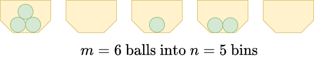
m balls are thrown randomly into n bins. The target bin for each of the m balls is determined uniformly and independently of the other throws.

Sounds easy enough, right? However, some famous mathematical, as well as computer science problems can be described and analyzed using this process. Among them:

1. Birthday paradox: If there are m people in a room, what is the probability of two of them having the same birthday? We assume that the birthdays are uniformly distributed over n=365 days.
   Translated into balls and bins: What is the probability that at least one of the bins contains at least two of the balls?
2. Coupon collector’s problem: A collector wants to collect all of n distinct stickers. Whenever he buys a package, he gets one sticker in a uniformly random and independent manner. What is the expected number of packages he has to buy to collect all n stickers?
   Translated into balls and bins: How many balls do we have to throw until all bins contain at least one ball in expectation?
3. Dynamic resource allocation: Important websites are not stored on merely a single but on n servers. That is because if one server crashes the website should still be available. One reason for a crash might be that too many of m people use the same server trying to access the website. But how to prevent that? It’s impossible to oversee millions of people acting independently and properly route them to servers with a low load in real-time, especially since these people don’t communicate with each other. One very easy way to do this is to uniformly distribute the users onto the n servers. But is it good? What is the maximum load of any of these servers?
   Translated into balls and bins: What is the (expected) maximum load across all bins after all balls were thrown?

Now, we will first analyze this problem and check out some interesting properties!

Quick Wins

Let us deal with the easy things at first. If you know a bit about probabilities, the following results should not surprise you.

The Number of Balls in a particular Bin

We have m balls. The probability of one ball landing in a particular bin is 1/n. Therefore, the number of balls Nᵢ bin i is binomially distributed with parameters m and 1/n for each i.

In particular,

• we expect m/n balls in this bin and
• the probability of the bin staying empty is (1–1/n)ᵐ.

The Number of Throws until a Ball lands in a particular Bin

Since each ball lands in bin i with probability 1/n, the number of throws until bini is not empty anymore is geometrically distributed with parameter 1/n.

We see that things are uncomplicated if you want to answer questions about single bins. However, most interesting questions, including the three aforementioned ones, involve statements about all bins at once.

Any bin with two balls? Does every bin have at least one ball? What is the maximum load of any bin?

The problem is that the numbers of balls in the bins are stochastically dependent on each other.

To demonstrate this, imagine that all of the m balls have landed in bin 1. The number of balls in bins 2 to n is determined now: it is zero. This dependence makes tackling the three problems from the introduction more difficult, but not impossible.

Harder Problems

Let’s take a look at the three problems from the introduction.

What is the probability that one bin contains two balls?

Probably you have seen this one in the birthday paradox setting with n=365 and something like m=23. We denote the event “all bins contain less than two balls” as E, the counter-event of what we actually ask for. Then you can argue like this:

• After the first throw, the probability for E is 1=1–0/n.
• The second throw is not allowed to land in the bin of the first ball, thus the probability for E after two throws is (1–0/n)*(1–1/n).
• The third throw is not allowed to land in the bin of the first two balls, thus the probability for E after two throws is (1–0/n)*(1–1/n)*(1–2/n).
• …

In total, we get

A small sanity check: For m>n the probability should be zero according to the pigeonhole principle. The formula above reflects this since the factor for m=n+1 is zero, thus the whole product is. Nice!

So the answer to our initial question is 1-P(E).

How many balls to throw until all bins contain a ball in expectation?

A simple argument is as follows:

• The number X₁ of throws until one bin is filled is Geo(1) distributed, i.e. after a single throw, one bin will be filled, obviously.
• From there, the number X₂ of throws until some second bin contains a ball is Geo(1–1/n) distributed since with probability 1/n a ball lands in the first filled bin again. But with probability 1–1/n, the ball lands in some other bin, the second filled bin.
• From there, the number X₃ of throws until some third bin contains a ball is Geo(1–2/n) distributed since with probability 2/n a ball lands in the first or second filled bin again. But with probability 1–2/n, the ball lands in some other bin, the third filled bin.
• …

Since a Geo(p) distributed random variable has a mean of 1/p, the expected number of throws until all n bins are filled is

where the sum is called the harmonic sum. For large n, it can be approximated by

where γ≈0.5772 is the Euler–Mascheroni constant. So, in total the expected number of throws is about n*(ln(n)+0.5772).

If you studied maths, you have probably encountered both problems and knew their solution already. At least it was like this for me. The third problem and its solution, however, surprised me.

What is the expected maximum load across all bins?

I will give you the solution to this problem without proof. Let Mₘ,ₙ be the expectation of the maximum in any bin. From the paper “Balls into Bins” — A Simple and Tight Analysis by Martin Raab and Angelika Steger, it follows for large n:

Especially the case for m=n got me. What I expected was a constant, maybe. If I throw a million balls into a million bins, I expect a few bins to stay empty, so of course, the maximum load should be larger than one. But here we see that it’s not just a constant, but a slowly growing function in n.

Now, what I want to tell you is the following: Solving these problems was definitely harder than the problems that deal with a single bin only. Especially for computing the expected maximum load, a lot of technical arguments are needed.

What I want to show you now is a method to deal with the balls into bins problem in a general way. As with everything in life, this comes with a price, unfortunately — looser bounds for the results we derive with this method. Furthermore, we cannot answer every question using this method. Let us see what this means.

The Poisson Approximation

The Poisson approximation method lets us upper-bound the probability of events in the balls into bins setting in an easy way.

The Method

The awesome book “Probability and Computing” by Michael Mitzenmacher and Eli Upfal recommends the following steps:

1. Pretend that the number of balls in each bin is independently Poisson distributed with parameter m/n.
2. Calculate the probability q of some event of your interest in this easier setting.
3. For the probability p of this event in the real balls into bins setting we have

where we call “e times the square root” the penalty factor.

Great, right? This implies for example, that rare events in the Poisson setting are also rare in the original setting.

This procedure is great because we don’t have to care about dependencies among the number of balls in the bins anymore. Everything is independent and following a simple Poisson distribution.

Of course, this inequality is not always meaningful, e.g. if q is a fixed number like 0.5. But if you can apply it, you can easily develop upper bounds for rare events without putting too much effort into the analysis.

You might ask: Why Poisson? And why m/n? A hand-waving argument is the following: We have said that the number of balls in a bin is Bin(m, 1/n) distributed. Such a distribution can be approximated (under certain conditions) using a Poisson distribution with the same mean, which is m/n.

Application to a New Problem

Let us consider the extended birthday problem as an easy example to solve with this method.

There are 20 people in a room. What is — at most — the probability that 3 of them share the same birthday?

This problem is hard to solve analytically. Try it yourself. Therefore, it’s a good playing ground for testing the Poisson approximation. Framed into the balls and bins setting:

20 balls are thrown into 365 bins. What is — at most — the probability of having 3 balls in one bin?

So, let’s do it the Poisson way. In the independent Poisson setting, and with m=20 and n=365 we have

Multiplying this with the penalty factor we get

Nice! This bound, however, is extremely loose. According to this site, the real probability is about 1%. This is due to the square root factor, which blows up the probability a lot.

But luckily, there is another upper bound without a square root factor! Also from the book “Probability and Computing”:

If the considered probability is increasing (or decreasing) in m, the penalty factor is 2.

If you think about it, you will see that we are in the increasing case. The more persons we have, the likelier it is to have 3 with the same birthday. Using the lower penalty factor, the Poisson approximation yields an upper bound of only 1.9%, which is close to the real probability of around 1%. Perfect!

Conclusion

We have seen an introduction to the balls into bins problem, which arises in several settings that do not seem related at first sight. It connects the birthday paradox with the coupon collector’s problem, for example.

Computing probabilities in this process can be cumbersome. Therefore, we have taken a look at the Poisson approximation for the balls into bins process. This approximation allows for easy computations of upper bounds of probabilities. However, these bounds might be quite bad since we get a rather large penalty factor. But there are also problems that require a smaller penalty factor of 2, as we have seen in the last example.

You can now frame some of your challenges as balls into bins problems and bound probabilities in this process using the Poisson approximation!

I hope that you learned something new, interesting, and useful today. Thanks for reading!

If you have any questions, write me on LinkedIn!