The Analyst’s Traveling Salesman Problem

The Traveling Salesman Problem is one of the great classic problems in mathematics. It’s easy to state, but trying to solve it is enormously hard (more on that later).

The papers written on it range from straight-up computer science to theoretical combinatorial optimization.

This article will describe a crazy twist on it: what if the set is infinite?

The Traveling Salesman Problem

The problem is fairly easy to state.

• Suppose you have a bunch of points.
• What’s the shortest path to hit them all?

The name of the problem comes from the idea of a traveling salesperson wanting to minimize the driving distance between a bunch of cities they would be visiting to make sales.

There are a few easy cases to think about. If you only have two points, then the straight line segment between them is the shortest path and the distance is the length of the line.

If you have three points, it’s pretty clear you still want to use straight-line segments (exercise: why?), and you can just brute force check all three possibilities to find the shortest.

I won’t go into all the history and difficulty of the problem. The main point is that it’s a hard problem. It’s NP-complete, which means that no computer algorithm can solve it “quickly.” (It’s outside the scope of this article to define what is meant by that).

Infinite Sets

Considering the classical problem has been an active area of research for 100 years, you might think there’d be no hope when we switch the problem from a finite number of points to any arbitrary (bounded) set.

But it turns out the problem is essentially solved in this case! The rest of this article will explain what is meant by this.

I’ll start with an example to prove that it even makes sense when we generalize because you’re probably thinking infinite things can’t have a “shortest distance.”

Example: Take any infinite collection of points on the line segment between (0,0) and (1,0). You could even consider all the points, which is uncountably infinite.

It doesn’t matter. The line segment itself touches every one of those points and it has length 1. This might seem like cheating, but it’s how we’re going to generalize the problem.

There should be at least two separate questions that immediately come to mind. Given an arbitrary bounded set E in ℝ²:

• Does there exist a finite-length (rectifiable) curve that contains every point of E?
• If so, what is the shortest such path?

The first question is basically a classification problem: which sets can we even hope to find a shortest path?

In mathematical terms we could rephrase this as: can we come up with necessary and sufficient conditions based on properties of the set itself to know if a finite-length curve passes through each point of the set?

The second question is “solving” the traveling salesman problem for these sets. In other words, actually calculating the shortest distance.

Remember, right now we’re making pretty much no assumption on the set E. This means it could even look like a crazy fractal.

Some Preliminary Examples

It’s easy to come up with examples to show that something more has to be said. For example, just take a filled-in square. There do exist weird “space-filling curves” that hit every point, but they don’t have finite length.

The fact that the square has a positive area rules it out as a possible set. This gives us the first criterion: we’ll only want to consider sets with dimension at most 1.

Here’s the construction of something called the four-corner Cantor set. (I described this in my last article, too).

If you’ve seen the construction of the Cantor set, then this should feel familiar.

Start with a square. Divide it up into a 4x4 grid and remove all but the four corner squares.

Now do that again with those 4 squares.

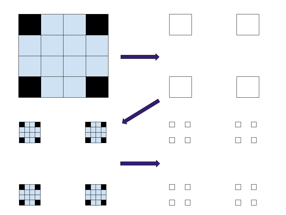
Keep iterating that process, and in the limit, you’ll end up with a set. This resulting set has Hausdorff dimension 1 (what we’re calling “1-dimensional”), and it is something known as a purely unrectifiable set.

First, it’s a process that results in something fractal-like. Second, we’re getting “corners” everywhere which makes the definition of a tangent impossible. If you aren’t familiar with purely unrectifiable sets, you can just think of those two properties as roughly the definition.

Sets with these properties have to also be ruled out just as a matter of definition. If there existed a rectifiable curve that passed through all the points, then it would be a rectifiable set.

These are some necessary conditions on E, but it doesn’t come close to solving the problem. Also, (Hausdorff) dimension is a slightly misleading concept here because there are 0-dimensional sets for which you can’t solve the problem!

The truly interesting part is to find some sort of quantifiable or numerical condition that doesn’t require us to actually produce the path or already know if a set is rectifiable by some other means.

Flatness When Zoomed In

Here’s the motivating idea: we want a number that tells us how far away from being “flat” the set is at various zoomed-in scales.

As usual, just think about the nicest types of sets first. If you start with a finite length differentiable curve, then the curve itself solves the traveling salesman problem for the set.

And this set has the really nice property of being flat (having tangent lines) when we zoom in:

But this is not necessary at all. In fact, it can be infinitely jagged all over the place and still be a curve that solves the problem. Just imagine the below picture is an iterated process of making the jagged parts where it goes on infinitely but in some convergent way:

We could easily make the thing have finite length but infinitely many non-flat points.

If you understand this idea, then you’re getting closer to the definition we need to consider for solving the problem in general.

Beta Numbers

What should it mean for a set to not be flat? Well, if we focus on a single chunk of the set and then consider every single line through that chunk, there’s always going to be a lot of points far away.

To see this, let’s take our set E to be an actual line (the black one) and the chunk to consider is just the part of the line through some box. We’ll think about all the possible red lines (only two are drawn, but there are infinitely many):

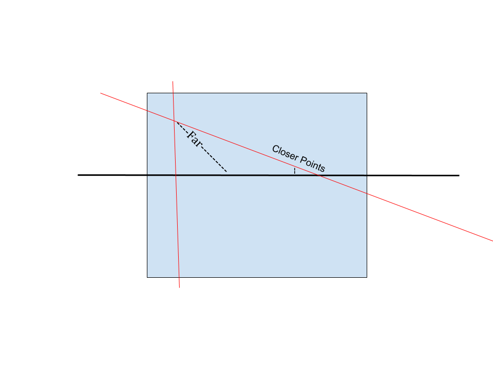
Our set/black line IS flat. But these two red lines still have some faraway points and some close points. This is just because we’ve picked bad lines to test the flatness of the black line. Once we start picking better and better lines, the number of faraway points goes to 0.

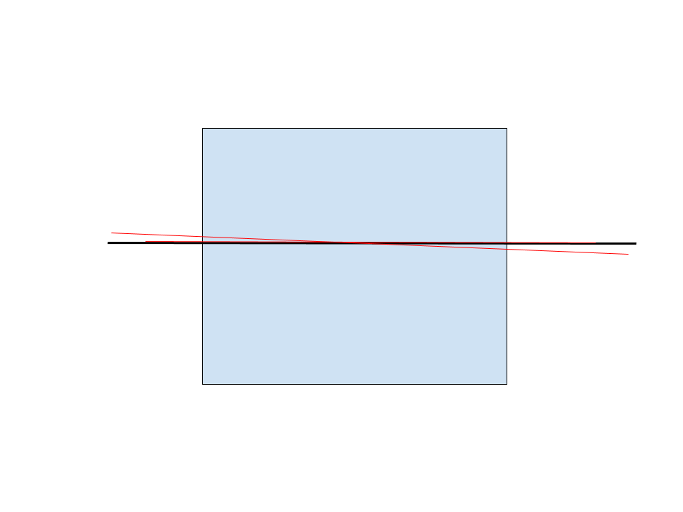
When we actually pick the line itself as one of the possible lines, all points are a distance 0 away:

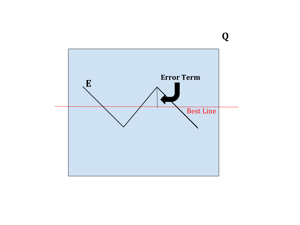
This brings us to the beta number of E on the scale of Q (a square). We consider all lines through the square Q. One of these will be the “best fit” in that the distances from E to the line are as small as possible.

We then divide that minimum error distance by the length of a side of Q (this is just “normalizing” to the amount we’ve zoomed in).

Before we formalize this, we should get more intuition. Note that this really is measuring the flatness somehow. The bigger beta is, the more not flat you look.

For a line, the beta is 0.

If you have a tangent line, the numerator of beta is the “error” of using the tangent line to approximate the curve. One of the foundations of Calculus is that this error gets smaller as we zoom in.

So, again, we can make beta as close to 0 as we want by making Q small in the situation of having tangent lines (being flat). Beta is 0 in the limit.

Error Terms

I’ll just rephrase the above in as compact a way as possible to make talking about it in the future easier.

The beta number of a set E on a square Q is just taking the line that approximates E the best and figuring out the worst “error” of this approximation (and dividing by the side-length of Q).

The technical definition is more complicated because there may not be a clear best line that does the approximation or an exact worst error, so you take an infimum over the set of all such things.

From now on, I’ll call these the error terms. This is a term I’ve made up for the article, so you won’t find it in the literature. We’ll label it e for error. The “length” of a side of Q is notated l(Q).

Thus, β(Q)=e(Q)/l(Q).

The Fundamental Concept

If all of this is a bit overwhelming, let’s take a moment to figure out why any of this might appear in the Traveling Salesman Problem.

First fundamental concept: beta was defined to be roughly 0 on Q when the set is flat and roughly 1 when the set is not flat on Q. This isn’t obvious, but it has to do with why we’re dividing by l(Q) in the definition of β.

Second fundamental concept: the Pythagorean Theorem is lurking in the background and will make all of this work.

Let’s consider a simple scenario where the set E consists of three points A, B, and C that are close to being flat:

The “best line” is just the line between A and C and the error is e, the length where you drop a perpendicular line from B.

Here’s the idea: we’d really like for our shortest path to just go A to C, but we have to go out of our way to hit B. I’ll call this a detour. The question is: how much length did we need to add to do this detour?

By definition, this excess length is a+b -(c+d). 
Rewriting this, it’s (a-c) + (b-d).

The Pythagorean Theorem says a²=c²+e². Let’s just do some basic factoring and rearranging:

a²-c²=e²
(a-c)(a+c)=e²
(a-c)=e²/(a+c)

Here’s a part people might not like, but we’re assuming this is relatively flat. In other words, β is small and hence a and c are fairly close in size. Let’s make an approximation now:

(a-c)≈e²/(2c)

Likewise, the same exact calculations on the other side show (b-d)≈e²/(2d). If B is placed roughly in the middle, then 2c≈2d≈(c+d).

This shows that the detour adds roughly e²/(c+d). If we’re using a square Q that is as small as possible to capture all three of these points, then the side length of Q notated l(Q) is exactly c+d, the denominator.

Let’s rephrase this in our notation. The detour adds a length of e(Q)²/l(Q) or in beta notation β(Q)²l(Q).

There are more sophisticated ways to keep track of the error terms and make the estimations without so many assumptions, but you should now believe that these numbers have something to do with how far off we are from making a straight line to solve the Traveling Salesman Problem.

P.S. If you want to make it more precise yourself, and you’re familiar with Calculus, try taking a square root at the Pythagorean Theorem step and use Taylor’s approximation. You’ll see you get the same answer but more rigorously.

Dyadic Squares

You may see where this is going now. I’ll jump to the punchline to keep your interest.

If E is just a flat line, we can go from one side to the other with no detours. In the above section, we saw that on a small scale, the detour we had to take was roughly e(Q)²/l(Q).

We might guess that if add up all the detours and get a finite “extra length” then we could solve the Traveling Salesman Problem for E (find a finite-length rectifiable curve that hits all the points of E), and this is exactly right!

This means we need a nice way to break up all of ℝ² into squares. The clever way to do this is to use dyadic squares. These are just the squares you get by taking side lengths of 2ⁿ (where n can be a positive or negative integer) and you have (0,0) be a corner.

If E is bounded, here are some facts:

• For some large n, there is a single dyadic square of side length 2ⁿ that covers the whole thing (this is basically the definition of being bounded). For all integers bigger than that, the error term is always the same.
• If we consider all dyadic squares, then we get arbitrarily small ones to capture the idea of zooming in to see flatness.

The Analyst Traveling Salesman Theorem

The Analyst Traveling Salesman Theorem (for ℝ²) was proved by Peter Jones in 1990. The paper was published in (arguably) the top math journal in the world to give you a sense of how big a deal this was.

Theorem: Given a bounded set E, there is a finite length (rectifiable) curve through E if and only if ∑e(3Q)²/l(Q)=∑β(3Q)²l(Q) is finite (where the sum is over all dyadic squares that intersect E).

Roughly speaking, the Traveling Salesman Problem can be solved for E if and only if these extra detours caused from not being flat can be added up at all zoomed-in scales and still be only a finite amount of “extra length.”

There’s some subtlety I’m leaving out for ease of reading here, like why 3Q appears and why the summation isn’t exactly the one shown on the Wikipedia page.

We should note that it’s an infinite sum, but the big squares eventually converge (the error is the same but the side lengths are 2ⁿ and calculus says that ∑(1/2ⁿ) converges).

This means only the small squares matter. But the small squares are just testing how “not flat” the set is, or equivalently, had bad the detours are going to be.

This is kind of amazing! It’s a single numerical criterion to tell whether we can solve the traveling salesman problem for crazy infinite and possibly fractal sets. This single criterion gives us both the necessary and sufficient conditions to do it.

We kind of figured that nice things with tangents would work, and that sum will definitely converge in that case (though it’s not as easy as it seems: try computing it for the unit circle, a doable but tricky exercise).

It turns out that there are lots of not locally flat things that also have finite length curves through them as long as this beta number/error term behaves nicely in the summation.

Jones actually proved more relating to the length of such a curve that solves the problem, but that’s outside the scope of this article.

So there you have it. This classical, very hard problem has actually been solved in this much more general setting!