Taylor’s Theorem

I’ve been putting this off for too long.

In several of my recent articles, I have taken advantage of the following result without much explanation:

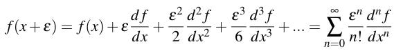
This is called the Taylor series expansion of f(x) about x. If ε is a very small number, then Taylor’s Theorem says that the following approximation is justified:

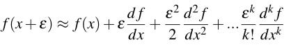
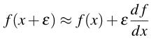
This is called a Taylor approximation to order k. The approximation for k=1, called the linear approximation, is especially important:

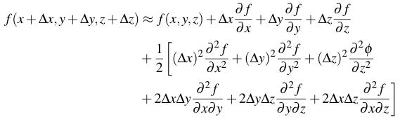
The approximation for k=2 is also sometimes used, for example in my last article on relaxation algorithms. The expansion is more complicated for multivariable functions so we’ll stop at second order for those:

I’m not going to prove Taylor’s Theorem in this article. That’s an elementary exercise that you can find in any calculus textbook and repeating it here would probably just bore you. YouTuber 3Blue1Brown has a pretty good heuristic explanation of the theorem itself:

Instead what I’m going to do is explain why it’s important in physics and go over two applications.

The need for Taylor’s Theorem

Taylor’s Theorem is used in physics when it’s necessary to write the value of a function at one point in terms of the value of that function at a nearby point. In physics, the linear approximation is often sufficient because you can assume a length scale at which second and higher powers of ε aren’t relevant.

For example, if at some point x we know the value of f(x), and we also know the value of f′(x), then we can estimate f(x+ε) by drawing the line through the point (x,f(x)) that has slope f′(x):

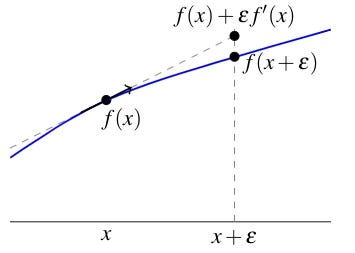
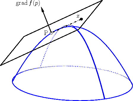
If the values of higher derivatives of f at x are known then this more detailed information about the behavior of f can be used to make a more accurate estimate of the value of f(x+ε). The generalization to multiple variables is obvious: just replace the tangent line with the tangent plane.

Taylor’s Theorem is also relevant in situations where we have some qualitative information about the relationship between physical processes at nearby points. That information can be expressed mathematically by associating the that qualitative information with the derivatives that appear in a Taylor expansion of a function that describes the process being studied.

An example arose in my recent article on the Navier-Stokes Equations. I had to find the relationship between the velocities of two test particles contained in an infinitesimal parcel of fluid. The information that I had was the empirical fact that the motion of a parcel of an incompressible Newtonian fluid has a translation component, a rotation component, and a component associated with the deformation of the parcel. By using a linear approximation to express the motion of one of the particles in terms of the motion of the other and interpreting the result, I found expressions for the translation, rotation, and deformation.

These are situations that you will encounter routinely in both theoretical and experimental physics. Introductory and intermediate physics courses don’t spend much time on Taylor approximation (or approximation techniques in general) because routine, simple problems with exact answers are more instructive at that educational stage than more open-ended problems that may require some creativity to solve, which may include strategic application of linear approximations. The case has even been made that physics itself is in some sense the study of linearization applied to the natural world. Whether you agree with this strong interpretation or not, the fact is that a working knowledge of Taylor’s Theorem and its consequences is absolutely essential to physicists and you will not get very far without it.

Example: The multipole expansion

Suppose that we would like to investigate the distribution of charge inside a sample of material. To accomplish this, we have to deduce information about the distribution by observing how it interacts with an electric potential. We assume that we have complete knowledge of the applied potential because this is our experiment and we get to control all of that. Our strategy will be to represent the unknown distribution as a superposition of elementary charge distributions each of which interacts only with the nᵗʰ-order terms in the Taylor expansion of the potential. Such a decomposition is called a multipole expansion.

Let ϕ represent the known potential and let ρ represent the unknown charge density function for the sample. Let V be the region occupied by the sample, and assume that this region is very small and includes the origin. The charges that produce ϕ are far away from the sample.

The energy associated with the interaction between the two collections of charges is given by the volume integral of ρϕ over V.

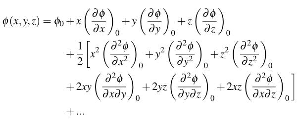
Let’s write ϕ as a Taylor expansion near the origin with ϕ₀ being the potential at the origin. Then the potential at (x,y,z) in V is:

The first term in the total energy will be:

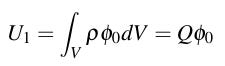
So the elementary distribution that interacts with the zero-order term in the expansion is a point charge at the origin whose value is the total charge of the sample. Another word for point charge is monopole, so we call Q the monopole moment of the sample.

For the next term, let’s start by making the following simplification:

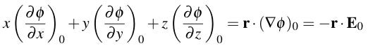
Where E₀ is the electric field at the origin due to ϕ. The interaction energy for this part is given by:

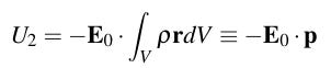
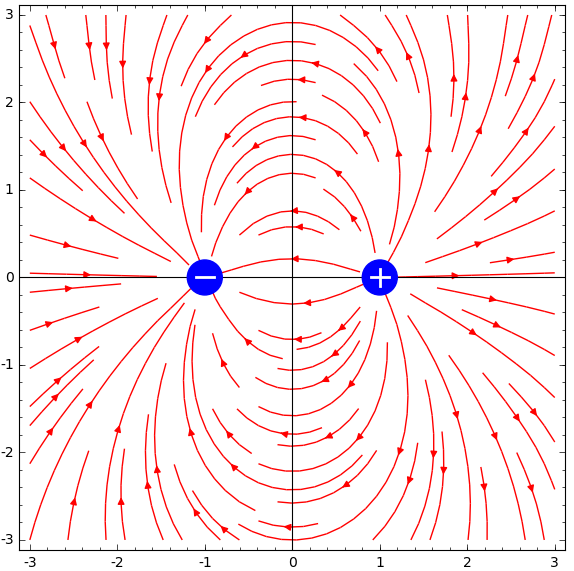
The integral of ρr over an entire distribution of charge is called the dipole moment of the charge distribution, labelled p. Therefore the elementary distribution that interacts with the first-order terms in the Taylor expansion of ϕ is a pure dipole with moment p. A pure electric dipole is a pair of equal and opposite charges separated by a fixed distance. If the distribution has a nonzero dipole moment then this means that there is a net separation of positive and negative charges along the line through the origin whose direction is that of the vector p.

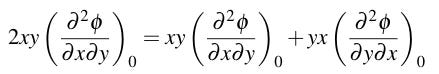
Now to simplify the remaining terms. Let’s start by separating the mixed partials, for instance:

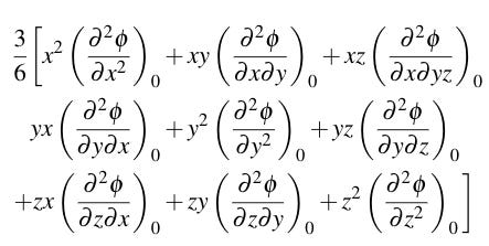
Now we replace 1/2 by 3/6:

None of the charges that produce ϕ are present in V, so ϕ obeys Laplace’s equation at the origin:

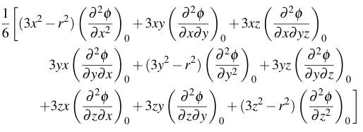
This means that we can add any multiple of (∇²ϕ)₀ to the sum of second derivatives without changing that expression’s value, so let’s add -(r²/6)(∇²ϕ)₀ where r²=x²+y²+z²:

Let i and j both be elements of the set of variables {x,y,z} and make the assignment:

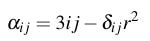
The symbol δᵢⱼ is called the Kronecker delta:

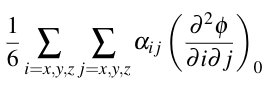
So for example if i=x, j=y then αᵢⱼ=3xy, or if i=j=z then αᵢⱼ=3z²-r². Then the sum of second partials takes the form:

Now we compute the energy integral for the second-order terms:

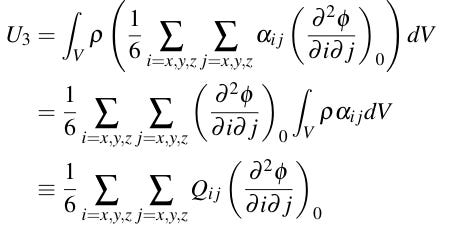
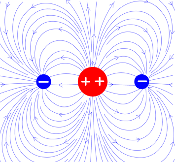
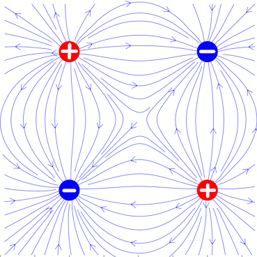
The integral of ραᵢⱼ over a distribution of charge is called the distribution’s quadrupole moment, which is a tensor represented as a 3×3 array whose components are Qᵢⱼ. Therefore the elementary distribution that interacts with the second-order terms in the expansion of ϕ is a pure quadrupole whose moment tensor has components Qᵢⱼ. A pure quadrupole is a pair of equal dipoles pointing in opposite directions. The quadrupole moment gives us information about the way in which the distribution deviates from spherical symmetry.

By continuing, we would find interaction energies for the sample’s octopole moment, 16-pole moment, 32-pole moment, and so on. In practice, the interaction energy of higher-order multipole moments decreases rapidly with increasing order so we often get a very good approximation by stopping at the quadrupole moment.

Therefore we can write the total interaction energy as:

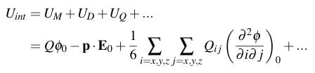
The values of the moments can be deduced experimentally by observing how the energy changes as ϕ is varied, and this gives us a mechanism for analyzing the internal electrical structure of a sample of matter.

This makes the theory of the multipole expansion important in molecular and atomic physics. For example, to determine whether a chemical has polar or non-polar molecules, test a sample of the chemical and see if it has a dipole moment.

An atomic nucleus’s shape can be inferred by measuring its quadrupole moment. It turns out that if a distribution is rotationally symmetrical about one axis, called the principle axis, then the quadrupole tensor has only one independent component, which we call Q. Context will prevent confusion with total charge.

If Q>0 then the distribution is stretched along the principle axis (prolate), if Q<0 then the distribution is flattened along the principle axis (oblate), and if Q=0 then the nucleus is spherical. Measurements of nuclear quadrupole moments have found that prolate shapes are much more common than oblate shapes. Explaining this remains an unsolved problem.

Example: Conservation of momentum and translation symmetry

Noether’s Theorem is an important result in theoretical physics that says, loosely, that if a system’s behavior does not change under a particular infinitesimal transformation then that transformation corresponds to a conserved quantity. We will show how translation symmetry leads to conservation of momentum. For simplicity we will assume that the system is conservative.

Suppose that a system consists of a collection of n particles, each at position (xᵢ,yᵢ,zᵢ). Let the potential energy be a function of the positions of all of the particles, V(x₁,…, xₙ,Y, Z) where Y and Z are shorthand for all of the y and z coordinates of the particles. Suppose that if every particle in the system is translated along the x-direction by an infinitesimal distance ε then V([x₁+ε],…,[xₙ+ε],Y, Z)=V(x₁,…, xₙ,Y, Z). We do not assume that this is true if only some of the particles are translated. For example, it will not be true if the potential energy depends on the distances between particles.

We make the following linear expansion:

Then from the assumption of translation symmetry:

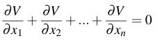
For conservative systems, F=-∇V so the sum of the x-components of the force on each particle is zero, meaning the system experiences no net force in the x-direction. Force is the time derivative of momentum, so the x-component of the total momentum is conserved.

Concluding remarks and copyright stuff

Approximation theorems aren’t that important in basic physics courses but they become more and more important as you start to learn advanced physics. Linear approximations in particular will find their way into nearly everything you do in advanced physics, so it is essential for you to be comfortable with them.

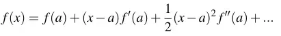
I should note that Taylor expansions are often written in a different form:

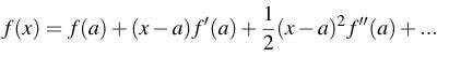
To get the form used in this article, replace a with x and x with x+ε. The form used is purely a matter of notation and one or the other may be more convenient for a given problem.

I have attributed all images that are not my own original work. Fair use guidelines protect the use of these images for purposes such as news reporting, criticism, and educational discussion.