Schrödinger’s Equation

Last time, we discussed the dual nature of matter, in which particles behave like waves and waves behave like particles. To explain this we introduce the wave function, which describes not the actual position of a particle, but the probability of finding the particle at a given point. Furthermore, when we consider the wave function as describing the state of a “probability field”, we see that the time-dependent behavior of this field exhibits wave-like behavior.

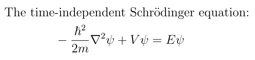
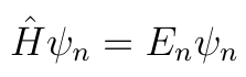
Suppose that the particle’s interactions with the world are represented by a potential energy function V(r) which depends only on the particle’s position. We will not address the case where V depends explicitly on time or on other variables. Then the aforementioned “probability field” is described by the wave function ψ, which satisfies a partial differential equation called Schrödinger’s equation:

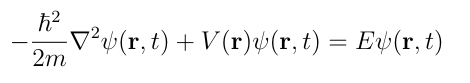
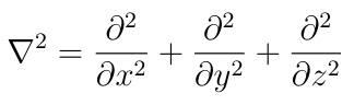
In this equation, r means position (x,y,z), ħ is Planck’s reduced constant, E is the total energy, and ∇² is the Laplacian operator:

If you know anything about partial differential equations (and if you don’t, then the article that I wrote last year about the heat equation might serve as a good primer: The Heat Equation, explained) then you know that in general this equation will be solved by an entire family of linear combinations of basis solutions ψₙ. These basis solutions represent what are called “stationary states”.

Let’s now make a brief digression into linear algebra. We can represent the left-hand side of Schrödinger’s equation by a differential operator called the Hamiltonian:

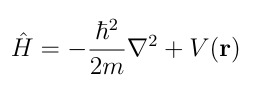
It is straightforward to show that this operator is linear. Therefore Schrödinger’s equation is an eigenvalue equation, which tells us that the energy Eₙ is the eigenvalue corresponding to the eigenvector ψₙ (we could also call ψₙ an eigenfunction):

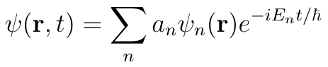
When the potential does not explicitly depend on time, we say that we are working in the “time-independent case”. This does not mean, however, that the solution has no time dependence. Time appears in the solution as a phase factor, exp(-iωₙt) where ωₙ=Eₙ/ħ. Furthermore, any linear combination of of eigenfunctions ψₙ will also be a solution to Schrödinger’s equation so the general form of the solution is:

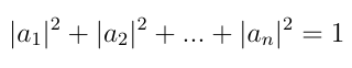
The aₙ are complex numbers which obey the normalization condition:

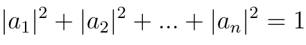
If the wave function is a linear combination of more than one eigenfunction ψₙ, then we say that the system is in a superposition of the states corresponding to the eigenfunctions appearing in the sum. If we take a measurement of the system, then we will find that it is in state k with probability |aₖ|² and the wave function of the particle will be ψₖ. The follow-up to this article will go into more detail about the formal meaning of the state of a system in quantum mechanics.

Probability and variables

When we specify the state of a system in classical physics, we are making a statement about the precise values of its dynamical variables, meaning quantities like position and momentum. This is not how it works in quantum physics. Instead, specifying the state of a system in quantum physics means specifying the probabilities that the dynamical variables will take certain values. Another point of divergence is that, unlike in classical physics, in quantum physics we need to deal with both discrete and continuous variables, and therefore with discrete and continuous probability distributions.

A discrete probability distribution will take the form:

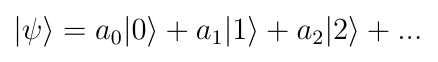
We have used Dirac’s notation here. The symbols |n〉 are called “ket vectors” or “state vectors”, and they represent the states of a system corresponding to the nth value of a discrete variable.The normalization condition applies:

In addition to ket vectors, there are also bra vectors (together they sound like “bracket”), and these are written as 〈n|. If we consider a ket vector |ψ〉 as a column vector, then 〈ψ| is obtained by transposing |ψ〉 into a row vector and then complex conjugating the components of |ψ〉. Since the product when a row vector acts on a column vector from the left is a scalar, we can use Dirac’s notation to define an inner product on the vector space spanned by the basis vectors |0〉, |1〉, etc. This vector space is called the “state space” or “Hilbert space”. Given two state vectors |ψ〉 and |φ〉, the inner product is 〈φ|ψ〉. We can use this inner product structure to impose an orthonormality condition on the basis states that we’ve chosen for the state space:

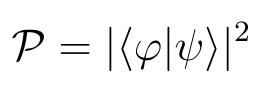
As a postulate, we will say that if a system is known to be in state |ψ〉, then the probability that a measurement will find the system to be in state |φ〉 is:

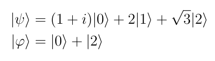
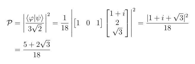
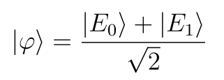
Let’s consider an example. Let|ψ〉 and |φ〉 be the following states:

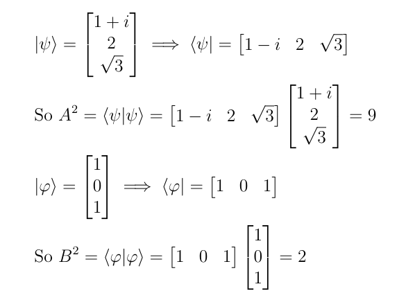
Let’s find the probability that the system that is known to have state vector|ψ〉 will be found to have state vector |φ〉 when measured. The first thing that we need to do is normalize the two vectors, that is, make |〈ψ|ψ〉|²=|〈φ|φ〉|²=1. To do this, we let A²=〈ψ|ψ〉 and then divide the coefficients in |ψ〉 by A. This will ensure that |〈ψ|ψ〉|²=1. The normalization constants are:

Therefore the probability is:

In this notation, we can write the series expansion form of the wave function as a state vector:

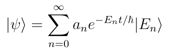
Suppose that we want the probability that the system has energy Eₖ for some particular value of k. Assume that the aₙ are already normalized. This probability is:

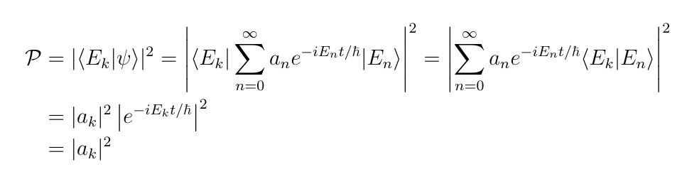
The phase factor disappears because the square of its absolute value is 1, and this lack of time dependence is why we call the states |Eₖ〉 stationary. On the other hand, suppose that the system has the following wave function:

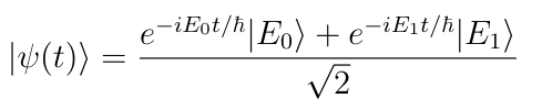
Suppose also that we want to know the probability that the system is in the following state:

This probability is:

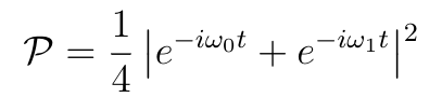
Remember that ωₙ=Eₙ/ħ. Remember that for a complex number z, |z|²=zz̄ where z̄ is the complex conjugate of z. Therefore:

So superpositions of stationary states are not necessarily also stationary.

That’s it for the discrete situation. The continuous case is much simpler. If a particle is in a state whose wave function is ψ, then the probability that the particle is in some region of space V is:

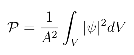
Where A² is the integral of |ψ|² over all of space. As a very simple example, consider the following wave function:

So now we’ve gone through an extremely brief outline of what Schrödinger’s equation is. But the best way to really understand physics is to do physics, so now let’s look at some examples.

The free particle

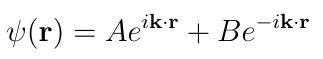
I’ve already covered the case of the free particle in my article on wave-particle duality, but I’ll briefly recap here. The particle is free in the sense that it is not subject to any external interactions, so V(r)=0. Schrödinger’s equation for the free particle is:

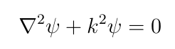
Where k² = 2mE/ħ². The solution is:

When we include the phase factor we get:

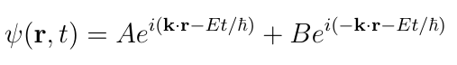
Where A² is the probability that the particle propagates in the direction of the vector k and B² is the probability that the particle propagates in the direction opposite to k. Remember that|k|²=k². Since the particle is free, this latter probability is zero and the solution is:

This solution tells us that free particles propagate like waves, which resolves the wave-particle duality paradox.

Particle in a box

We will now find the stationary states for a particle subject to an infinite square well potential:

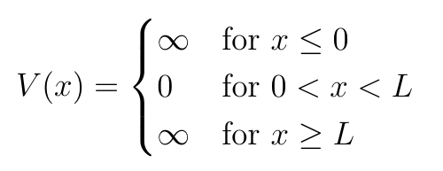
If the particle was anywhere outside of the well from -L/2 to L/2, then it would have infinite energy, which is not physically possible. Therefore the probability for the particle to be anywhere outside of the well is exactly zero. Therefore we need to solve the problem for the one-dimensional free particle:

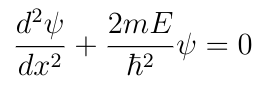
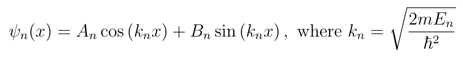
This will be subject to the boundary condition ψ(0)=ψ(L)=0. From elementary differential equations, the stationary states must have the following form:

The stationary solutions need to satisfy the following two equations:

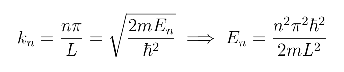
Since sin(0)=0, the first line means that Aₙ=0 for all n. Then the second line reduces to Bₙsin(kₙL)=0. This could be satisfied by Bₙ=0, but Aₙ=Bₙ=0 gives the trivial solution, which is not interesting to us. The other possibility is kₙ=nπ/L, which works because sin(nπ)=0 for all integers n. Therefore we have a formula for the energy levels:

To finish things off, we need to find Bₙ. We can’t use the boundary conditions since we’ve already used them to solve for Eₙ. Fortunately, the other condition that must be solved by the solutions is normalization. Therefore:

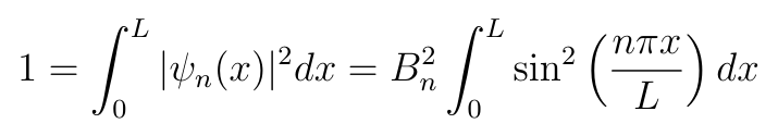
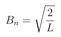
By computing the integral and solving for Bₙ, the solution is:

Therefore the possible states of a particle trapped in an infinite square well potential are represented by:

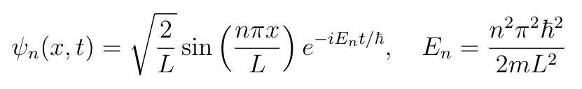
This result tells us two interesting things:

• First, it demonstrates quantization of energy. Any particle in the box must have an energy at one of the given values.
• Second, the minimum energy is not zero. If it was zero, then n=0, and therefore ψ=0, so the probability of finding the particle anywhere in space is zero, meaning that the particle does not exist.

The particle-in-a-box is mostly an instructional example, but it does have real applications. The same basic reasoning that we’ve used here also applies in any situation where a particle is confined to a small region but is free to move around within that region. For example, one can obtain useful back-of-the-envelope results by representing the particles of an atomic nucleus or the conduction electrons in a piece of metal as particles in a box.

Quantum tunneling

Consider a ball resting at the base of a hill of height h. The ball is kicked so that it has an initial speed v₀ and initial kinetic energy mv₀²/2 and begins rolling up the hill. As the ball rolls up the hill, it has to work against gravity, so kinetic energy turns into gravitational potential energy and the ball slows down. When the ball reaches height y, the amount of kinetic energy that has been lost to gravity is mgy where m is the mass of the ball and g=9.8m/s² is the constant acceleration due to uniform gravity. If for some y<h, mv₀²/2=mgy, then the ball runs out of kinetic energy, stops, and begins rolling back down hill. On the other hand, if mv₀²/2>mgh, then the ball has enough kinetic energy to overcome gravity and cross the hill.

The hill is a kind of potential barrier: a region of space containing a force field that can only be crossed by particles that have enough kinetic energy when they enter the barrier. In classical mechanics, a particle either does or does not have enough kinetic energy to cross the barrier. But in quantum mechanics, a particle with kinetic energy less than the “height” of the potential barrier still has a chance to end up on the other side. This is called tunneling.

We’ll consider a rectangular potential barrier, which has the following form:

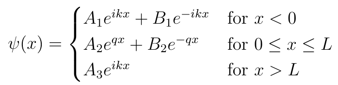
Suppose that a particle approaches from the left with kinetic energy E₀<V₀ We’ll calculate the probability that the particle will end up on the other side of the barrier. This probability is called the transmission coefficient T. To do so, we need to solve for the wave function piecewise in the three intervals x<0 (region 1), 0≤x≤L (region 2), and L<x (region 3). In regions 1 and 3, the particle is free, and we’ve already solved for the wave functions in this case:

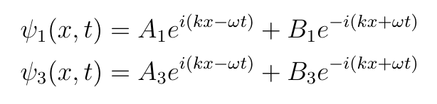
Where A₁ is the amplitude for a particle in region 1 traveling to the right, B₁ is the amplitude for a particle in region 1 traveling to the left after being reflected back from the potential barrier, A₃ is the amplitude for a particle in region 3 traveling to the right, and B₃ is the amplitude for a particle in region 3 traveling to the left. Clearly B₃=0 because no particles are approaching the barrier from the right. Now we need to find the wave function inside the barrier. Schrödinger’s equation is:

Where V₀-E₀>0. Now we’ll rearrange a little:

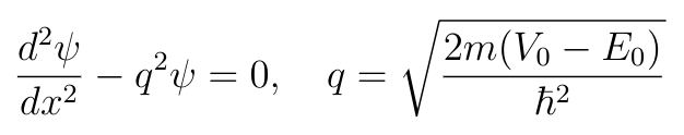
Remember that q is a real number. From elementary differential equations, we know that the solution is:

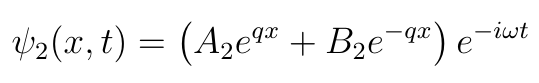
Where we have also remembered to include the phase factor. However, since as we can see all of the wave functions are in phase with each other, we can drop off the phase factors and just write the general solution as:

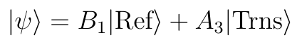
Recall that we said that B₁ is the amplitude for a particle to be in region 1 and to be traveling to the left and A₃ is the amplitude for a particle to be in region 3 and to be travelling to the right. The only reason that a particle would be in region 1 and traveling to the left is if it was reflected from the barrier, and the only reason that a particle would be in region 3 and traveling to the right is if it tunneled through the barrier.

Let’s now use that information to represent the state of the particle as an abstract state vector which is a superposition of the states “transmitted” and “reflected”:

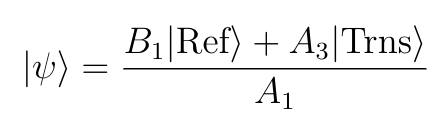
As always, the first thing we do when presented with a state vector is to normalize it:

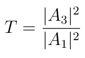
The term in the denominator is amplitude for the superposition of both possible outcomes, meaning that it’s the amplitude for either event to occur without concern for exactly which of the two. A necessary condition for this is that the particle must first have been incident on the barrier, and being incident on the barrier is also a sufficient condition because transmission and reflection are possible. Therefore a particle will be transmitted or reflected if and only if it is incident on the barrier, so the total amplitude in the denominator is equal to the amplitude of an incident particle, meaning that:

So the transmission coefficient is:

Now to solve for A₁ and A₃, we’ll use the fact that ψ and dψ/dx must both be continuous at x=0 and x=L. This gives us the following system of equations:

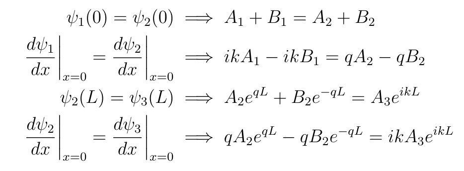
It might seem as though we’re stuck, because this is a system of four equations involving five variables. But we’re only interested in the ratio A₃/A₁ so this is not a problem for us. To do this, we’ll use the third and fourth equations to solve for A₂ and B₂ in terms of A₃, and then we’ll plug the result into the first two equations to find A₃/A₁.

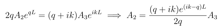
To solve for A₂, multiply the third line by q and then add the fourth line to the third to obtain:

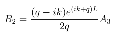
Similarly for B₂:

Eliminate B₁ from the first equation by multiplying the first equation by ik and then adding the second line to the first and then substitute our results for A₂ and B₂:

Now take the absolute value of both sides, square, and take the reciprocal:

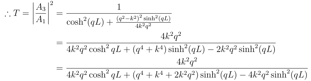
By using the fact that cosh²(x)-sinh²(x)=1 and rearranging, we find that:

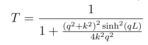
And then we get T in terms of the energy and potential by substituting q and k:

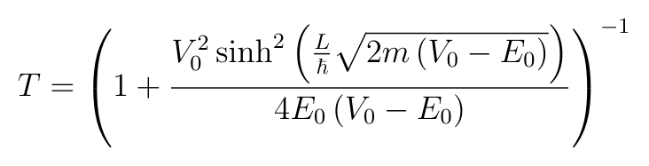
The reflection coefficient can be calculated from R=1-T.

Interestingly, there is a kind of dual phenomenon to quantum tunneling. Just as an incident particle with energy less than the height of the potential barrier has a nonzero probability to cross the barrier, there is also a nonzero probability that an incident particle with energy greater than the height of the potential barrier will be reflected.

Tunneling is among the most important quantum mechanical effects, both in the natural world and in technological applications. For example, if tunneling did not occur, then electrostatic repulsion would almost always prevent atomic nuclei from ever coming close enough to fuse, and therefore nuclear fusion would be practically impossible. Tunneling also places important limitations on the sizes of modern semiconductor devices: if the electronic components are too small, then it becomes difficult for them to operate useful because electrons may simply tunnel past them.

But one of the most striking examples is the scanning tunneling microscope, invented in 1981 by Gerd Binnig and Heinrich Rohrer in 1981 and for which they were award the 1986 Nobel Prize in physics. In the STM, a small, sharp, conductive tip is held at a fixed height just above the surface of the sample and scans along the surface:

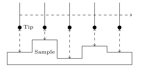
The gap between the tip and the sample acts as a potential barrier. If the sample is closer to the tip, then the potential barrier is smaller, and more electrons will be transmitted. By counting the number of electrons transmitted at each point, the height of the sample can be determined, and this can be used to create a picture of the surface at a resolution that can show the positions of individual atoms:

Closing remarks

This article took longer to write than expected. The main reason was that I wasn’t sure how best to go about introducing Schrödinger’s equation. In particular, I was not sure whether it would be best to approach via a more rigorous formalism since that’s what makes the most sense to me or to keep things simple and focus on demonstration. In the end, I decided that the best thing to do would be to do both: write one article (this one) where I simply show what Schrödinger’s equation is and what it does, and then write a sequel where I explain what’s actually going on. I alluded to this briefly in the second section when I name-dropped Hilbert spaces. In the follow-up, I will have much more to say about this.

I have cited any images that are not my own original work. Fair use guidelines protect the use of this material for purposes of reporting, instruction, and criticism.

UPDATE 02/16/2020: When this article was first uploaded, the picture of Schrödinger’s equation in the thumbnail and in the header of this article was missing the negative sign on the ħ²/2m term. I apologize for this mistake.