Relaxation Methods

This article will introduce a powerful class of numerical analysis techniques called relaxation methods in the context of electrostatics and fluid dynamics.

Let ϕ be a function of x and y and let A, B, …, G also be functions of x and y. Any second-order partial differential equation with ϕ as its solution may be written in the form:

The subscripts represent partial derivatives, for example ϕₓ=∂ϕ/∂x. We have 2B instead of just B because ∂²ϕ/∂x∂y=∂²ϕ/∂y∂x. In this article, we will be interested in PDEs where B²-AC is strictly negative. Such PDEs are called elliptic.

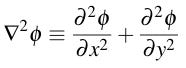
One of the simplest elliptic equations is Poisson’s equation ∇²ϕ=f(x,y). The special case ∇²ϕ=0 is called Laplace’s equation. The operator ∇² is called the Laplacian:

Since B=0 and A=C=1, it is clear that Laplace’s and Poisson’s equations are elliptic. Poisson’s equation is important in the study of electrostatics because it arises from Gauss’s law: since ∇⋅E=ρ/ε₀ and E=-∇ϕ we have ∇⋅E=∇⋅(-∇ϕ) resulting in ∇²ϕ=-ρ/ε₀, where ρ is the charge density function. Laplace’s equation therefore applies in regions of space in which there are no charges, for example between the plates of a capacitor.

Laplace’s equation also occurs in fluid dynamics. If a fluid’s velocity field V is irrotational then ∇×V=0 meaning that V is conservative and therefore there exists a function ϕ such that V=∇ϕ. Taking the divergence of both sides gives ∇⋅V=∇²ϕ. Then by the continuity equation -∂ρ/∂t=∇²ϕ where ρ is the density of the fluid. If the fluid is also incompressible then ρ is constant so ∇²ϕ=0. This potential has units of m²/s.

In this article, we will be solving Laplace’s equation in regions of space bounded by surfaces on which ϕ is known. A problem of this form is called a Dirichlet problem for Laplace’s equation.

Solving Dirichlet problems analytically can be time-consuming even for simple boundary conditions and for many realistic boundary conditions it often just isn’t worth the effort to pursue an analytical solution. Consequently, many numerical approximation schemes exist for solving Direchlet problems, and relaxation techniques are an important classes of those schemes. A relaxation scheme, broadly speaking, approximates the solution at each point by writing it as a simple function of its neighboring points.

The simplest way to construct a relaxation algorithm for solving Laplace’s equation is to impose a square grid onto the region of interest where points are separated by their neighbors by distance h, and then approximate ϕ at (x,y) by its average over the points (x+h,y), (x,y+h), (x-h,y), and (x,y-h). We can confirm that this will give an accurate approximation by using Taylor’s theorem. First, write out the Taylor expansions of ϕ for the nearest neighbors on the grid:

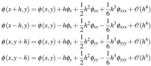
The symbol 𝓞(h⁴) means terms in which h appears with fourth power or higher. By adding together these four equations and moving ϕ(x,y) over to the left we obtain:

The expression attached to the h² is just the Laplacian and since ∇²ϕ=f this term becomes h²f. Furthermore, as h approaches 0, fourth and higher powers of hvanish much more quickly than the h² term. Therefore when h is very small relative to the length scale of the problem, the higher power terms vanish and the following approximation is valid:

So much for the math part, now let’s talk about the relaxation algorithm itself. Note that in this article we will only consider boundaries consisting of lines parallel to the x and y axes, such as in the example below where the black dots would indicate grid points spaced 1 centimeter apart.

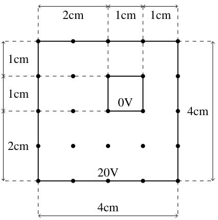
More complicated geometries involving smooth curves or non-right angles are beyond the scope of an introductory article. For simplicity, we will also assume that f=0.

I will use MATLAB in my examples since it is particularly well-suited for this. If you do not have MATLAB and want to play with the code yourself then you can use Scilab, a free and open source clone of MATLAB that is compatible with simple MATLAB code. Keep in mind that in MATLAB, (1,1) indexes the top left element of an array and (i,j) is the element in row i and column j.

The procedure is as follows.

• Initialize an (M+1)×(N+1) rectangular array called phi(i,j) where M and N are the width and height of the area being modeled divided by the grid spacing. For example, in the above picture the width and height are 4 centimeters and the grid spacing is 1 centimeter, so M=N=4. Assign boundary values to the relevant points.
• For all points (i,j) that are not on the boundary, PHI(i,j)=0.25×[PHI(i+1,j)+PHI(i-1,j)+PHI(i,j+1)+PHI(i,j-1)]
• Stop after the desired number of iterations or level of accuracy is reached.
• If desired, MATLAB and Scilab both have built-in routines that can plot the result.

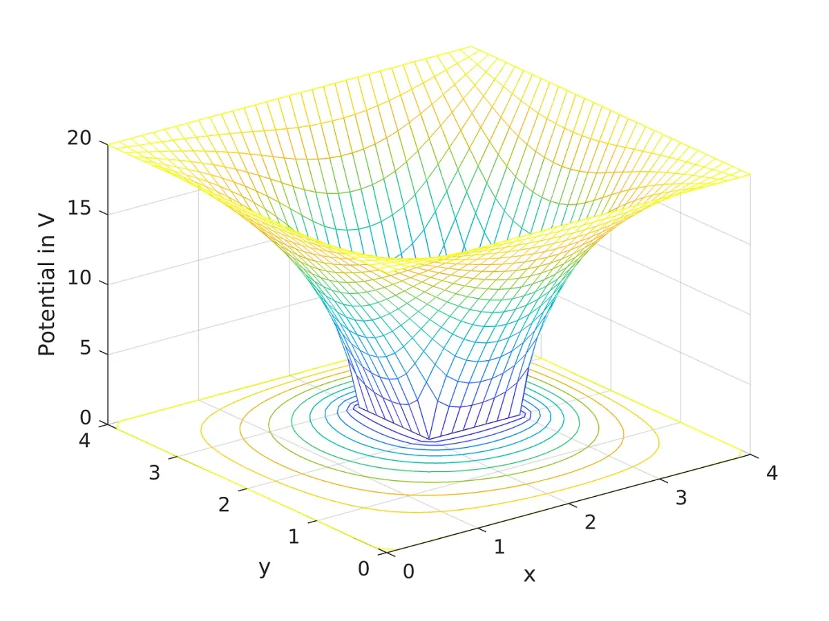
The next two images are the result of applying relaxation to Example 1 with the grid spacing set to a more practical 0.125 centimeters. To avoid cluttering the article, I have put the code on Pastebin. You may find the comments in the code useful if you want to experiment with it. The code should work in Scilab.

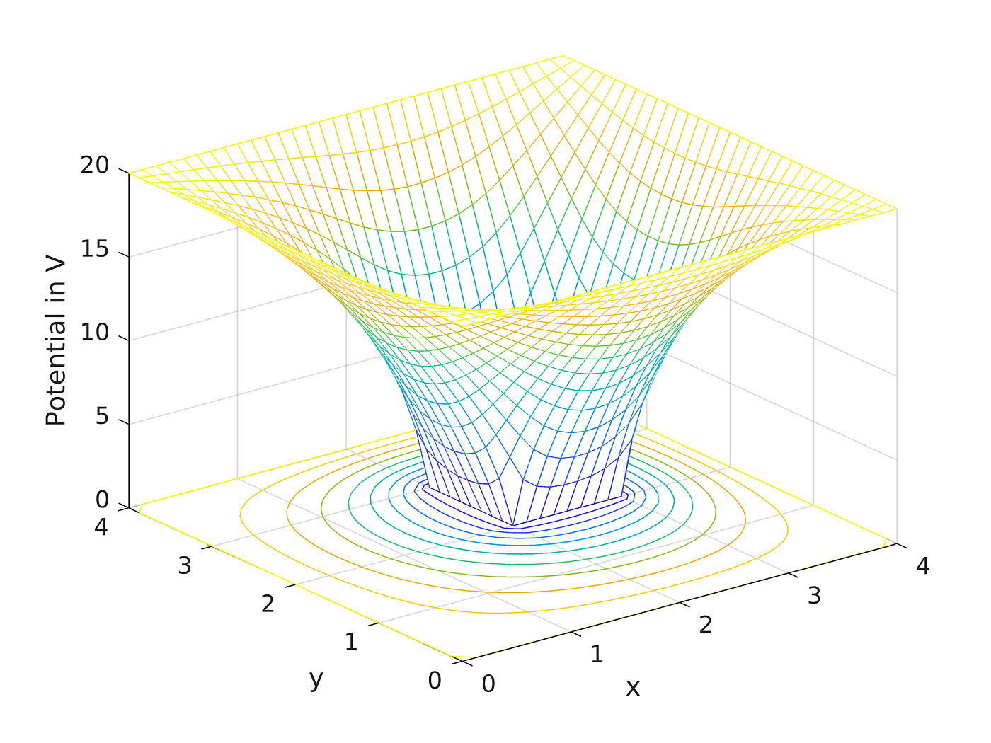
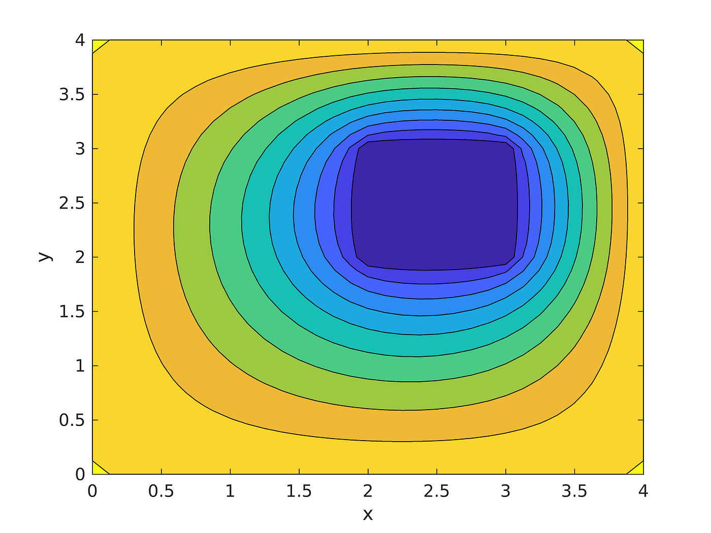
These images also illustrate the screening property: A region enclosed by a grounded conductor is completely isolated from external potentials. However, it is not necessary for the region to be completely enclosed in order to achieve good protection from interference. This is the principle behind the Faraday cage.

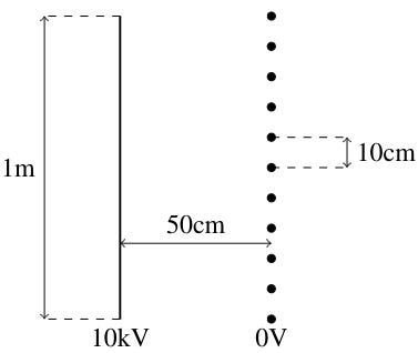
A one-meter long plate is held at 10kV and a Faraday cage consisting of centimeter-thick bars, with 10 centimeter spacing between them, is placed 50 centimeters from the plate. The code that I wrote for this example is here.

Let’s first see what it would look like without the Faraday cage.

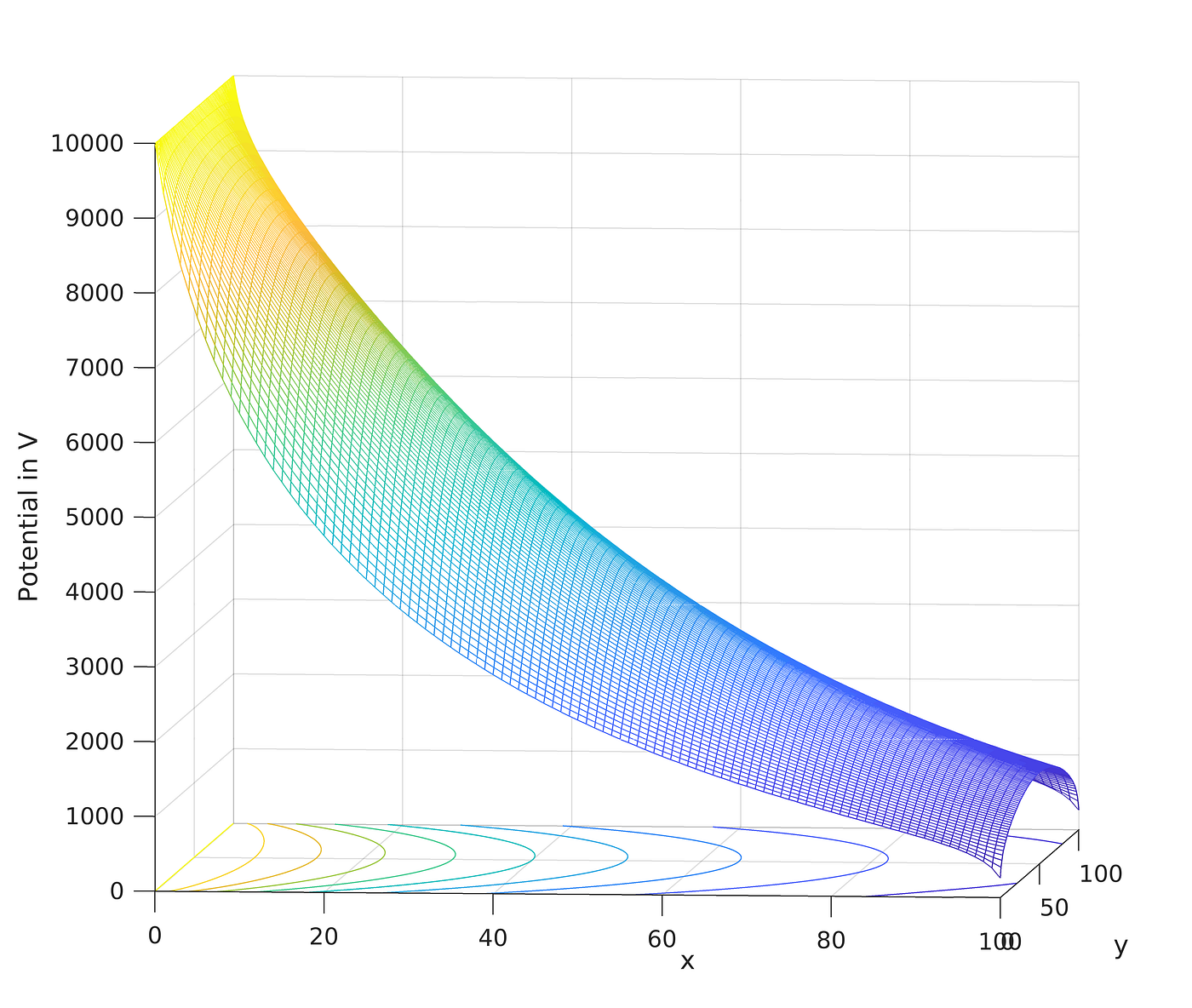
As expected, the potential decreases approximately linearly with increasing distance from the plate and would converge on being exactly linear if the plate were to become infinitely long in the y-direction. Now let’s add the cage.

You can see that the cage makes an enormous difference even though it does not even come close to perfectly separating the two regions. Now let’s look at an example from fluid dynamics.

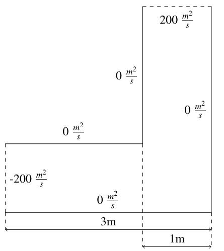
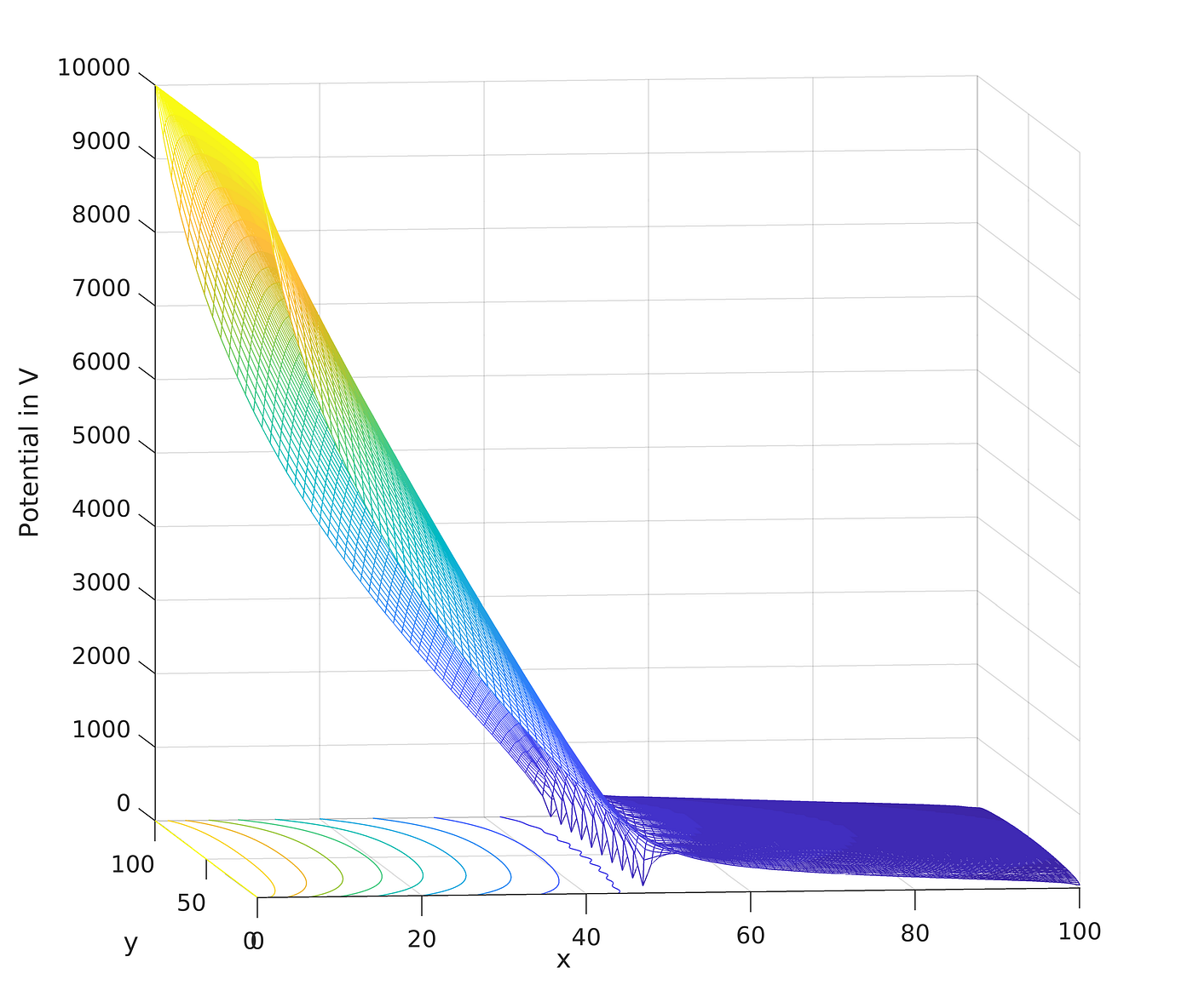
The ends of a 1 meter wide L-shaped pipe, measuring 3 meters on its sides, are held at 200m²/s and -200m²/s and the walls are held at 0m²/s. Let’s find the flow in the pipe. Since V=∇ϕ, the velocity is in the direction of increasing ϕ, so the bottom left boundary at -200m²/s represents the inlet to the pipe and the top left at 200m²/s represents the outlet.

The code for the relaxation is here. This is the graph of the result:

An interesting feature of this potential is that it is very flat near the corner, and this occurs even for extremely large values of the potential at the outlet and inlet. This is related to the skew-symmetry of the boundary conditions about the line y=300-x. We can interpret this graph as saying that a test particle immersed in the fluid that comes into the pipe in the middle of the bottom left corner (say at x=0, y=50) is initially moving quickly, then it lingers for a while when it reaches the corner section, and then speeds up again as it moves towards the outlet in the top right. A streamline plot shows some of the trajectories, although not the speed of the particle at each point on its trajectory:

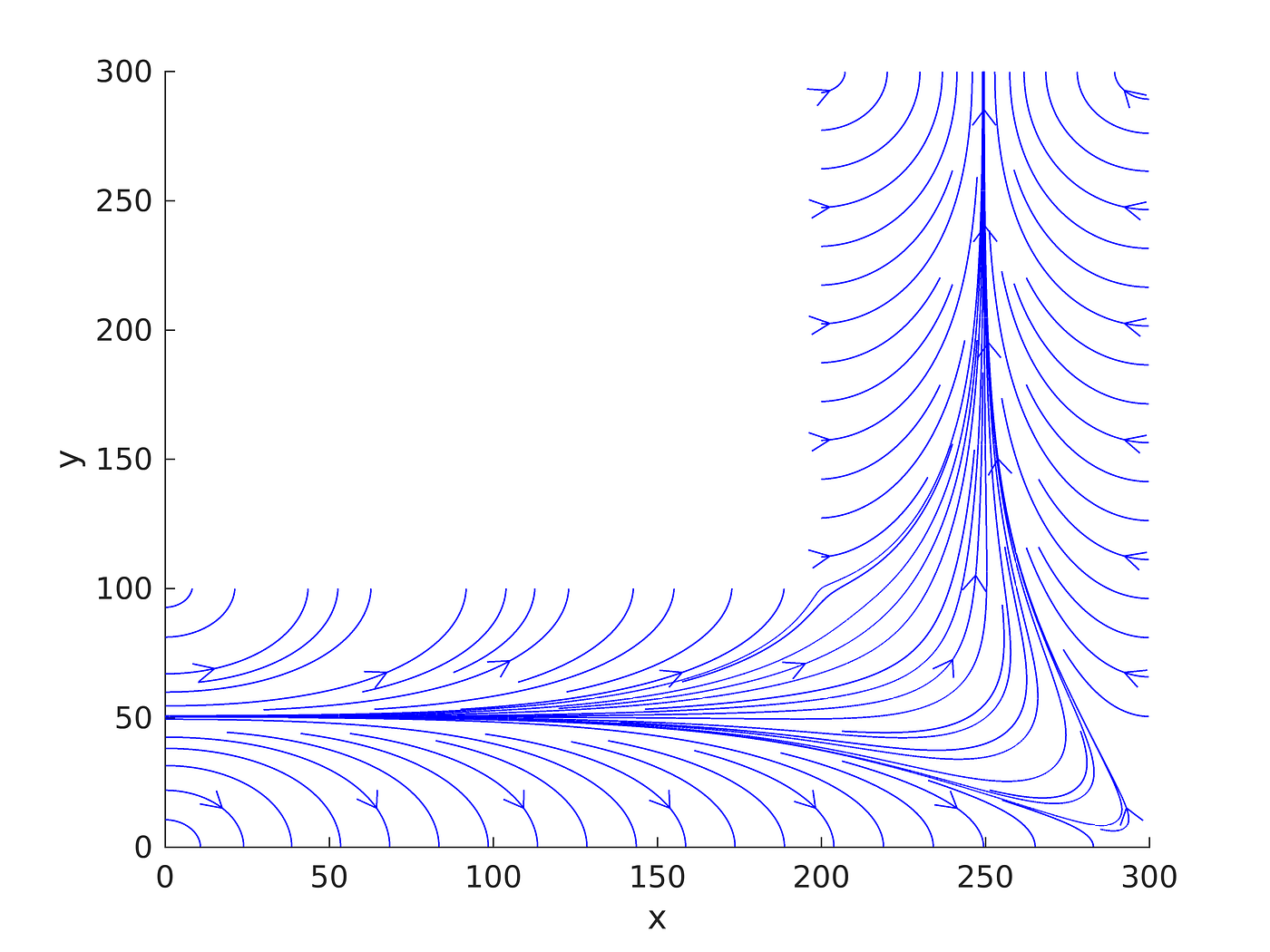
Another interesting behavior is that in the horizontal section of the pipe, test particles are pushed into the wall, and in the vertical section they are pushed away. The streamline plot does not show this, but particles will not actually stop when they hit the wall, but will instead travel along the wall on a path approximately parallel to the wall. Likewise, particles do not originate at the vertical walls, the streamlines pointing away from the walls represent particles that had been flowing along the walls being pushed away.

This solution is the least accurate of the three that I have presented. In particular, the shape of the streamlines is more sensitive to the length of the grid spacing than is the shape of the mesh plot of the potential. Unfortunately I’m stuck using my 2011 Macbook Air until I can afford a new computer so I could not make the spacing as small as I would have liked, but if you happen to have a more powerful computer then I would highly encourage playing with the settings in the MATLAB code. In particular, I would recommend trying a 0.1 centimeter separation as opposed to the default value of 5 centimeters.

Concluding remarks

It would be nice if we could always analyze physical systems analytically so that we could obtain perfectly accurate solutions, but in the real world that just isn’t possible. This is why numerical techniques are so important to physicists and engineers, and any aspiring professional in either of these fields will be expected to have at least a basic working knowledge of numerical methods.

Those interested in further reading might find this article, which was the inspiration for Example 3, illuminating.

Copyright stuff and other disclaimers

All images in this article and code that I linked are my own original work and I don’t mind if you want to share or use them as long as you attribute them to me. I give permission — in fact, I encourage it — to download, run, and modify my code. However, while MATLAB and Scilab are very safe and compatible with most modern computers I cannot promise that my code will work perfectly for everyone.