The Task

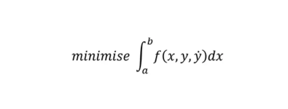
We are going to tackle a problem. The journey we take solving it will teach us how to differentiate ‘with respect to a function’, and even understand the Fundamental Lemma of Calculus of Variations. (Crikey).

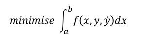
We are given the function f, and want to pick a function y such that we minimise the integral. In the next section I will give a real world example to help you understand what this means and why it is helpful.

As you go through, try and understand the intuition and key ideas on a first reading, and don’t be too concerned if not every detail makes sense.

You will need an understanding of some of the ideas behind single variable calculus to understand the equations, but I explain in words most of the key concepts.

Motivation.

Suppose we have an automated rocket, and we fire it into the sky at a point x = a. We want it to hit the ground at x = b and we want to minimise the cost of getting from a to b. In real life, we might have considerations like not smashing into other planes or making sure we land the right way up.

We get to choose its path, i.e. what y(x) is: the height of the rocket at each point of the ground it flies over. But there are some restrictions. Obviously, we cannot teleport, so y(x) must be continuous (this sort of means you can draw the path without taking your pencil off the page.*) Also, we cannot change our speed must change smoothly — so the derivative of y must be defined. Note that it might change very rapidly, but it cannot jumpy in an infinitesimally small amount of time, which seems reasonable. (For instance, when you sprint and speed up, you accelerate quickly, but you don’t suddenly skip from 5 miles an hour to 7 miles an hour, you have to accelerate through all the intervening numbers. So your acceleration can jumpy but your speed can’t, and your position certainly can’t jump!)

Now, we are going to make a slightly bizarre assumption. But it turns out to be a crucial one in making this problem tractable.

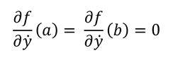
If this expression doesn’t make much sense to you now, then don’t worry, as it will later. I give a mini-explanation below if you can’t wait.

f is a function of three variables. f(x,y,z)
The derivative of f with respect to z is defined.
Instead of z, we have dy/dx. This is a bit confusing at first.
However, f doesn't care that dy/dx is a function. All it cares about is the number put into the z slot, and how its output changes as the input to the z-slot changes. So pretend dy/dx is z. What we are then doing is evaluating this expression at the endpoints, a and b, and asserting that they must be equal to zero.

This assumption isn’t too crazy. At the very end we are flying low, we obviously aren’t going to be using lots of fuel to accelerate. In any case, tying down our function at two points still gives us lots of room to make it a reasonable choice, so the restriction isn’t very big.

We want to transport our rocket cheaply as possible. This is represented by the function inside the integral, which converts all these variables into how much it is costing us per small unit of time. For example, the higher we are up in the air, the atmosphere is thinner. To accelerate upwards means moving against gravity, while going accelerating downwards is easy because of gravity.

The integral sums up all these costings.

*there is a technical definition of continuity, which is important when looking at functions which are very strange and continuous.

But how on earth do we solve this?

We don’t want to maximise or minimise any particular function. Instead we need to pick the function.

At this point, it might occur to you that we want to differentiate a function. At least, this is what occurred to me after several hours of head scratching when first worked on this problem over the summer.

Suppose that we had found our unique minimal solution. Then, if we were to ‘perturb’ our function with another function, h, scaled by an arbitrarily small epsilon, then the resulting function should get larger.

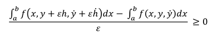
What does this expression mean?
y describes our original flight path. y-dot is the derivative of this. the curly e stands for a very small number.Suppose your intern suggests a new flight path h(). The rocket is expensive, so you decide to adjust the path slightly as the intern recommends, scaling their flight path by the very small number 'epsilon' or curly-e. The cost of the new flight path is the LHS integral, and our old flight path cost is the RHS integral. The curly-e on the bottom is to rescale, like a normalising constant, the the magnitudes are sensible.If we have found our best path, your intern's suggestion will increase the cost, even if we only slightly adjust in the direction they want. The intern goes back to making coffee, and you go back to being the super-genius rocket scientist.

What we are saying here is ‘suppose we had found our solution. Then for any small changes we make to that function, the cost increases’. This is basically the definition of what it means for our function to minimise our cost!

We are about to use a Taylor series.

Crash course in what a Taylor Series is. Featuring: you, your car, and your children screaming in the back. A Taylor series basically says: for any function, we can use its local rates of change to get a good approximation. If I tell you a car’s location and speed, I’ll have a pretty good idea of where you will be in 1 seconds time. If I tell you a car’s location, speed and acceleration, then you might have a good idea of where it is in 3 seconds time, or a really accurate knowledge of where it is in 1 seconds time. If I tell you the location, speed, acceleration and the rate at which you are easing off the gas pedal, you’ll be able to make an okay estimate for 10 seconds time, but your estimate for 1 seconds time will be brilliant. This is what we are about to do. The advantage is that location, speed, acceleration and gas pedal pressure are quite simple and easy to manipulate. In contrast, modelling the entirety of the human brain and your screaming kids in the back to fully recreate the travel experience may give a better predictions if you could pull it off but for manipulating the math in practice it’s impossible. The genius of taylor series and calculus is that as the time scale gets very small our approximation becomes infinitely good, so we can find out true results from what were previously just approximations.

When our perturbation is very small, we can use a Taylor series, taken from regular calculus. We now switch perspectives, and view the expression above as varying in epsilon (the wavy-e or squiggly e). In line with the example given earlier, our intern suggests an adjustment to the trajectory you worked out, and you get to decide to what extent you adjust in line with their recommendations. The expression below gives a good approximation to the adjusted path when we only change by a little — and as the adjustment gets very small, the estimate gets better and better.

Okay, I admit this is kinda scary, so let’s break it down.

As x varies over the range a to b, remember that x, y(x), h(x)are just NUMBERS. For instance, if a = 0 and b = 1, at x = 0.2 we might have:

y(0.2) = 0.1
h(0.2) = 0.9
y-dot(0.2) = 1
h-dot(0.2) = 3f is a function with three arguments. Evaluating f(x, y(x), y-dot(x)) at x = 0.2, we get:

f(0.2, y(0.2), y-dot(0.2)) = f(0.2, 0.1, 1)

We perturb to f(0.2, 0.3 + 0.001*0.09, 1 + 0.001*3)

All we have done is plug in the relevant numbers. As the perturbation is suitably small, we can apply our taylor series approximation. In the example above, the perturbations are only 0.00009 and 0.003 respectively, so our use of a Taylor series approximation is sensible. (if this terminology makes you feel uncomfortable, what we are doing is the same as the car example, where we know the position, speed and acceleration and want to predict where the car is in, say, 0.00009 seconds)

People normally get confused by the fact that the bottom half of the derivatives have functions as their arguments. Just pretend that it is a z or a w or some other variable. Then remember that the Taylor series approximation is valid for small perturbations around one of its arguments, and the derivative is defined around that argument. It doesn’t really matter what that argument is! A function is okay! At each point the function takes a value, just like a variable does. So for our current purposes, when the function is ‘bound’ within the integral, it really is no difference from a variable.

Some Fiddly Details (Optional)

Unfortunately, some of the bits below are more technical than intuitive. This is sometimes the case in mathematics. An understanding of integration by parts should give you a shot at understanding this, if you want to give it a go. Feel free to skip to the next section where we will see a beautiful and intuitive result.

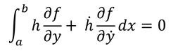
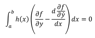
From this, with a bit of fiddly around with the specifics (doing the subtraction and dividing by the epsilons**), we can deduce that, for any function h(x)

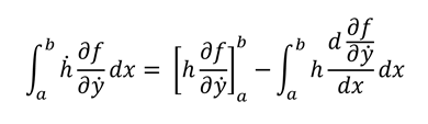
Using integration by parts on the RHS expression, we write the following.

We assume that, as seen near the beginning.

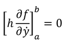
So we can write, for a given function h(x)

This isn’t very useful… (yet)

Now for some magic

In swoops The Fundamental Lemma of the Calculus of Variations. Let’s give an informal statement, and then give the technical definition.

Informal statement

You are calculating the area under a curve, and the area is equal to zero. This means that the curve is equal to zero everywhere, or there are some ‘mounds’ of positive area and some ‘mounds’ of negative area, which cancel.

Now say that you can draw any new function, at each point you multiply it with the old function, and the area of these two functions multiplied is equal to zero.

We then say that our original function must be zero everywhere. (There will be graphs and examples below the technical statement)

Technical statement (Optional)

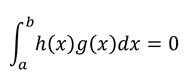
We want to prove that, if for all continuous functions h(x)

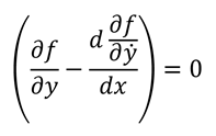
Then for all x on [a,b]

Despite the big name, this actually isn’t too hard to understand. To see why, write

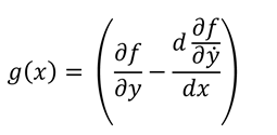
Replacing our complicated with g(x) gives us the statement of the Fundamental Lemma of the Calculus of Variations)

Then we have, for all continuous functions h(x)

Proof (Visual)

Suppose g(x) was not zero for some x. Then draw a mound shape, with h(x) very close to zero except in the region where g(x) is not zero. Where g(x) is not zero, make h(x) curve sharply up to one and down again. The resulting integral will not be zero.

Visually you can see this below. While g(x) (drawn in green) is sometimes above zero and sometimes below zero, by drawing h(x) (drawn in blue) appropriately, the function h*g (which is in purple) clearly has a positive area underneath it.

The Final Condition

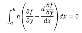
We have reduced the problem to solving the differential equation

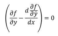
From here, we can go no further without more information about our function f. However, this is a substantially easier problem to solve. In particular, we can solve differential equations numerically, by plugging in small intervals (while I challenge you to find a nice way to numerically solve our original problem!).

If you have made it this far, thank you for your determination and patience!