A vacuum is a space with as little energy in it as possible. However, a vacuum is not entirely empty. It contains quantum fields. Quantum fields are obtained after the quantization of classical fields, which are functions of spacetime coordinates (such as, for example, the electromagnetic field). Mathematically quantum fields are operator-valued functions of space and time.

There are two types of vacuum: a true vacuum (or true ground state), which is a stable configuration of quantum fields located at the global minimum of the potential energy, and a false vacuum (or false ground state), which is a metastableconfiguration of quantum fields that occupies a local minimum instead of theglobal one. The instability is rendered by barrier penetration via quantum tunneling (classically, both vacua are stable).

The false vacuum was chosen to be zero for convenience. This article is based mostly on Coleman. I will explain why there is a probability that the vacuum state of our Universe is a false vacuum. If that is the case, it might undergo a tunneling transition to the true vacuum, the consequences of which would be catastrophic. In this transition, which is caused by quantum fluctuations, a bubbleof true vacuum would form. If the bubble is large enough it is (classically) energetically favorable for it to grow and spread “throughout the universe converting false vacuum to true.”

As pointed out by the celebrated American theoretical physicist Sidney Coleman, this probability is nonzero because our Universe is not “infinitely old” (if it were, the vacuum decay would have happened already). After the big bang, the Universe was far from any vacuum state (since its energy density was gigantic). As it cooled off (with the expansion) it may have “chosen” the falsevacuum (instead of a true vacuum). If the Universe got stuck there, the calculation of its decay probability is crucial if one wishes to predict its future behavior. Quoting Coleman:

“In the true vacuum, the constants of nature, the masses and couplings of the elementary particles, are all different from what they were in the false vacuum, and thus the observer is no longer capable of functioning biologically, or even chemically.”

— Sidney Coleman

We will therefore calculate the decay probability (per unit of time per unit of volume) Γ/V. We will see that to zeroth order in h it has the form:

where A and B are theory-dependent coefficients.

As will be shown in this article:

“Typically, we would expect [the initial radius of the bubble] to be a microphysical number… This means that by [our] standards, once the bubble materializes it begins to expand almost instantly with almost the velocity of light. As a consequence of this rapid expansion, if a bubble were expanding toward us at this moment, we would have essentially no warning of its approach until its arrival. At time 0.000000000000000000001 seconds [after the observer notices the bubble], he is inside [it].”

— Sidney Coleman

A Helpful Analogy: Nucleation Processes in Statistical Physics

In boiling superheated liquids, a similar phenomenon happens. As the liquid is heated, it settles in a metastable state of liquidity (instead of evaporating). The false and true vacua correspond, respectively, to the superheated liquid phase and to the vapor phase.

Thermal fluctuations (instead of quantum fluctuations — see above) result in the continuous materialization of small bubbles of gas in the liquid. Since inside the bubble is the true vacuum (with lower energy density) its presence lowers the total energy of the system. However, the surface energy of the bubble increasesthe energy of the system. Eventually, a large enough bubble will materialize so that it is energetically favorable for it to expand (in contrast, small bubbles tend to shrink and disappear). It will then convert the available liquid into vapor. See Lancaster and Blundell or Coleman for more details.

Quantum Tunneling for Particles

Though we will need quantum fields to explain the tunneling of the Universe, it is helpful to consider tunneling in non-relativistic quantum mechanics first.

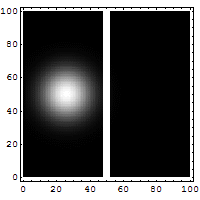
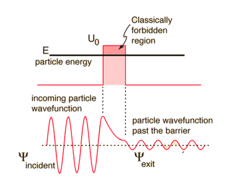
Let us consider a particle tunneling (see Fig. 5 and Fig. 6) through a potential. This is an essentially quantum phenomenon (a classical particle will rebound). The figure below shows an electron wave tunneling through a potential barrier. The dim spot on the right represents the electrons that crossed the barrier.

For a particle with total energy E in a region with potential V (see Fig. 6) the tunneling rate has the following form (to zeroth order in h):

Note that a prefactor was omitted.

The details about the tunneling are indicated in Fig. 7:

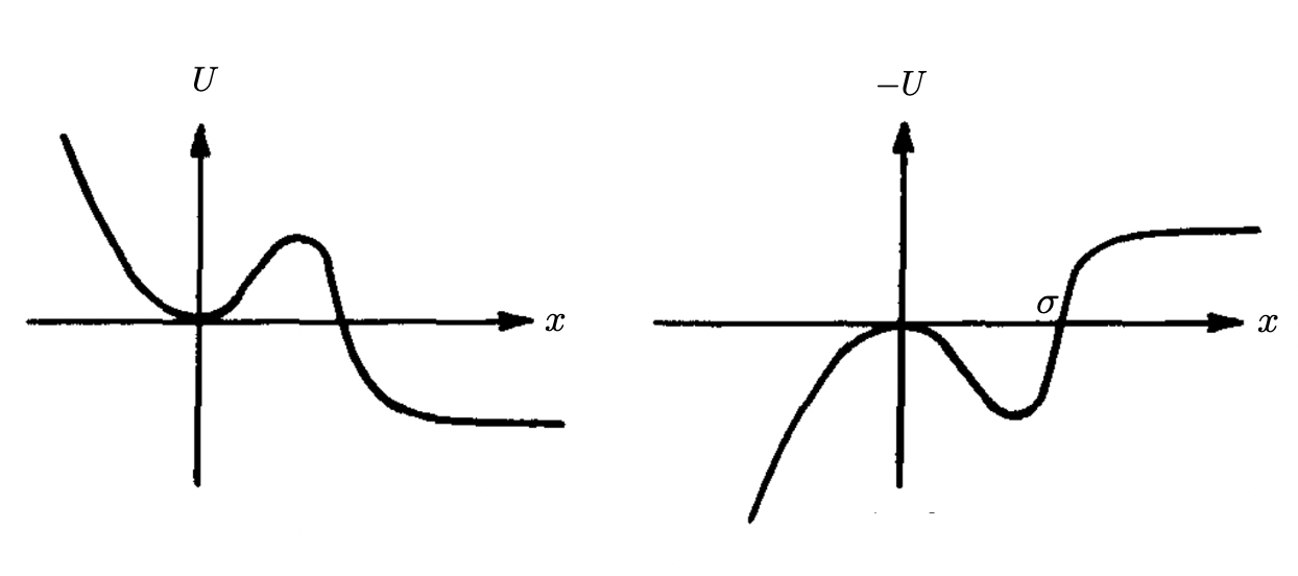
Let us now follow Coleman and consider the following potential (on the left of Fig. 8):

The Lagrangian reads:

Using the WKB approximation, we obtain the tunneling rate associated with the crossing of the potential barrier:

It is trivial to generalize the calculation to many dimensions. The Lagrangian becomes:

The coefficient B is given by:

where U(x₀)=0 and σ is a surface of zeros Σ. The integration is over the path that minimizes B:

After crossing the barrier the particle motion becomes classical (initially with zero kinetic energy).

According to Jacobi’s formulation of Maupertuis’s principle

with fixed endpoints. This equation determines the shape of the particle’s trajectory in the configuration space. These trajectories are solutions to the equations of motion:

Comparing Eq. 7 and Eq. 8 we notice that both variational principles differ in two aspects: in Eq. 7, E=0 and the signs of the potential are flipped. Since Eq. 7 corresponds to Eq. 10, Eq. 8 gives us:

Eq. 10 can be obtained from Eq. 9 via a transformation known as Wick rotation:

The variable τ is called imaginary or Euclidean time and the R subindex + indicates that τ >0.

Eq. 10 is the equation of motion obtained by extremizing the Euclidean Lagrangian:

The following two conditions are obeyed by x(τ):

A few observations about these conditions:

• The system is at its classical equilibrium point at τ → -∞
• The system is time translation invariant. Hence we can choose σ =0. At Euclidean time τ = 0, U=0. The second condition in Eq. 13 is obtained from Eq. 10.
• The second condition indicates a reversal of motion for τ > 0. This is a bounce off Σ at τ = 0. At τ → +∞, the particle returns to its classical equilibrium point.

From Eq. 9 and Eq. 12, we also have:

Using these results we obtain from Eq. 6 the value of B:

We will now translate our procedure to the quantum fields.

False Vacuum Decay in our Universe

Let us return to the problem described in the introduction (the metastable vacuum of the Universe) and use the last section to calculate the decay probability. Consider, for simplicity, a quantum scalar field with the following Euclidean action:

The bounce is a solution of the corresponding Euclidean equation of motion:

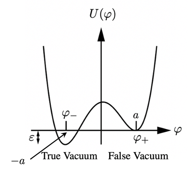
The following potential U(φ) will be used in the calculations:

where the first term is φ-symmetric and the false vacuum, chosen by the Universe, lies ε ≪1 above the true vacuum (see Fig. 2). Following Coleman, we define:

There are three bounce boundary conditions. The first condition states that the bounce solution goes from the false vacuum at -∞ back to the false vacuum at ∞. Mathematically it is expressed by:

The second condition is necessary for the Euclidean action or (or equivalently, the coefficient B)

to remain finite. It reads:

The third is:

which corresponds to the second condition in Eq. 13. As described in the introduction and will be discussed in detail shortly, these equations describe the formation of a bubble of true vacuum. According to Eq. 20, these bubbles are localized in space. Far from them, the system is still in the false vacuum.

Since the equation of motion and the boundary conditions are O(4) invariant (invariant under rotations in Euclidean four-space) it makes sense to suppose that the field depends only on the distance from the origin of four-space which is the radial variable:

This supposition was eventually proved in this paper. Eq. 16 becomes:

The conditions the field must obey are:

The second condition must be obeyed to avoid a singularity at ρ = 0 in the equation of motion for φ(ρ) above. As noted by Coleman, this method is extremely powerful since it reduces the problem of barrier penetration in a system with infinite degrees of freedom to the study of the properties of a single classical differential equation.

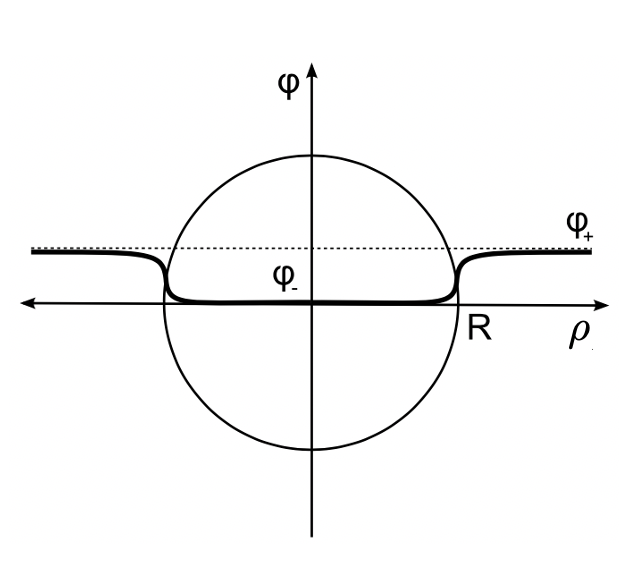
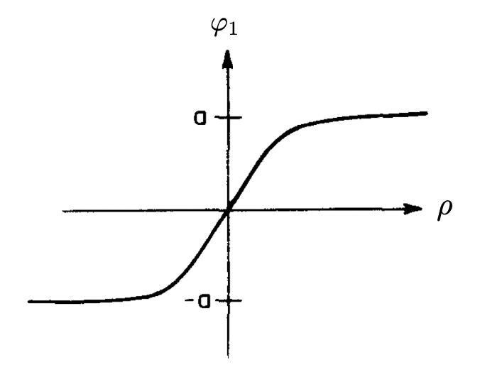
Note that if the solution to Eq. 23 is interpreted as a particle position and ρ as time, the equations of motion are identical to mechanical equations for a particle moving in a potential with flipped sign U → -U subject to a viscous force inversely proportional to time. According to Eq. 24, the particle is released at rest at time ρ=0. If its initial position is appropriately chosen, the particle will come to rest at t =∞ at φ=a (on the top of the hill where φ=a in the figure below). The existence of this initial position φ₁ is proved in Coleman.

Let us understand the form of the bounce. First, we choose φ(0). It must be very close to -a. Suppose it stays there for a very long time, until ρ ≡ R→ ∞. When ρ is close to R, it quickly rolls across the valley in Fig. 10 and slowly comes to rest at a (at t → ∞). In the field-theoretic language, the particle bounce looks like a four-dimensional static bubble of large radius R, with a thin wall separating the false vacuum outside it from the true one inside it.

We will now calculate B. Close to the boundary ρ = R, we have 3/ρ ≈ 0 and we can drop the viscous term in the equation of motion. Let us also set ε→ 0. Eq. 23 simplifies to:

which is the classical equation of motion for a particle in a symmetric double well. It has a one-dimensional instanton as a solution. Solving it we obtain (see details in Coleman):

Using the following equation for the symmetric part of U:

we obtain:

The action becomes:

The three regions of the bounce are:

The values of R and B are obtained by varying the Euclidean action with respect to R. We obtain:

Going to Minkowski Spacetime

As in the particle case, the field φ makes a quantum jump to the state

This gives the shape of the bubble after it is materialized in three-dimensional space. After the jump, its time evolution becomes classical:

Note that this equation is obtained merely by Wick rotating τ. Hence its solution is the bounce after the same transformation, namely:

As the bubble expands, its wall evolves as a hyperboloid:

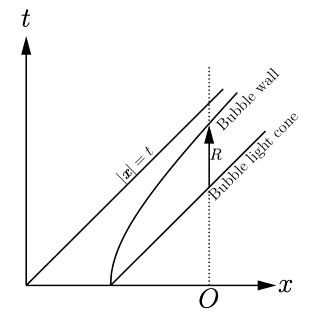
The observer O only notices the bubble when he crosses the bubble lightcone. After time R the observer is inside the bubble (notice that c is set to 1). As noted in the introduction,

Thanks for reading and see you soon! As always, constructive criticism and feedback are always welcome!

My Linkedin, personal website www.marcotavora.me, and Github have some other interesting content about physics and other topics such as mathematics, machine learning, deep learning, finance, and much more! Check them out!