There are a lot of reasons why I’m writing this, one of them is I could never understand Borel Sets, I got introduced to them on day one of my adventures in Probability Theory, there was something about the way it was portrayed, it didn’t make sense to me, like at all. So I broke it down into subconcepts, which I tried to tackle, but still nothing. There was nothing intuitive about them, or at least I couldn't see it. So, I skipped over it, which by the way you shouldn’t do, but it's almost helpful sometimes. But, I came across it again, sometime back when I was reading about Joint Probability Density Functions, so I investigated it. A couple of pointers before reading, you will need a good knowledge of probability at least high-school probability, a good grasp on set-notations. I apologize for switching to LaTEX quite often, it’s just easier to write math there also grammar mistakes, sorry about that.

What Is Probability?

If you read any literature on probability theory with the definition of probability you learned in high-school, you won’t get anywhere just because it is way too simple and shallow, to encapsulate the actual meaning of probability, now I’m not saying it’s wrong or anything, but with the definition which I will provide in this section, we can easily generalize it to anything you want.

So let’s start, for now, forget the definition of probability you know, we will start from the basics, which are made up of two things a Sample Space and an Event Space.

Sample Space: It is a collection of sets containing all the possible outcomes of an experiment. It can be finite(tossing a coin 2 times) or infinite(tossing a coin till a head shows up).

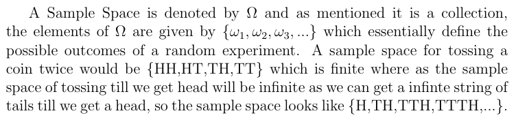
Now, these were examples of a discrete sample space, and surely you can imagine a continuous sample space as well but continuous here means that there is a range of possible outcomes, but an outcome can only be one. For example, the height of human beings, so as much as data you collect height of a human can only have a feasible range, like from 2 feet to 8 feet. But for this piece, you just need to understand discrete Sample spaces, that’s it.

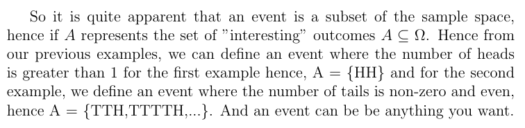
An Event: It is the subset of the sample space, to which we assign a probability measure, I know I haven't defined a “probability measure” so for now, we will define an event as an outcome that we are interested in.

Now that we have some knowledge about the things we are working on, we can introduce some entities that will aid us in understanding the space we are working in.

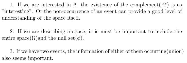
This is called an algebra, I know very misleading, but it’s formally called that so can’t do anything, but you can see we are describing these rules for a new collection. So let's formally define an algebra.

So we can call an arbitrary collection is an algebra if it follows the above three rules. And there are a lot of inferences that you can gather from these rules, one of them is that the algebra is closed under finite union and intersection, and I encourage you to think about why that is true. But just defining an algebra isn’t adequate, let’s take the second example, we cannot define the event A, which is the set that contains even number of tails preceding the head just by performing finite union or complements, we need to scale the union from finite to infinite. This introduces the notion of a σ-algebra. The description of a σ-algebra is the same as the definition of algebra, but with one key difference.

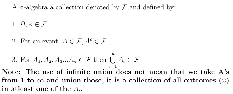
Also in rule 3, the number of A’s should be finite, only then we say σ-algebra is closed under countable infinite union.

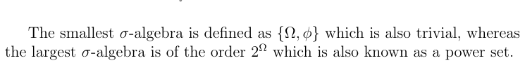
So now if we have a power set, and Ω is countably finite or countably infinite we can assign a measure to each ω the belongs to the events, an example of countably finite power set is tossing of coins, and an example of an un-countably infinite set is the range of [0,1]. Read this for more information on countable sets.

So now that we know we can assign a measure on a countably finite set, so let’s do that. But before we do that we need to look into some measure theory. I won’t go into much depth on this because it is out of scope for the article and frankly I don’t know a whole lot about it. So the only thing we require here is the notion of a measurable space. The definition of a measurable space stems from σ-algebra itself, so a pair (X, F) is called a measurable space if X is a set and F is the σ-algebra of the subsets of X. In our case, (Ω, F) is a measurable space, hence we can define measures on it. So the definition of a measure is as follows,

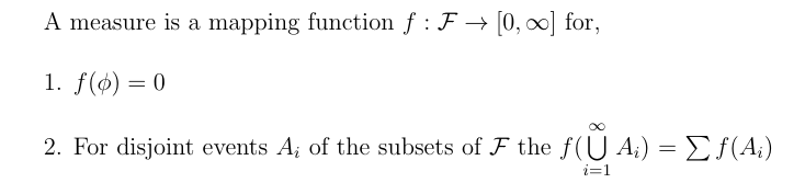
Now if you look closely, we are mapping our σ-algebra to the Real number line, and it satisfies the given two rules. Another observation is that this looks very similar to the rules of probability you might have studied. But before we jump to that, let’s break the above statements down. So it is evident, f(ϕ) = 0, so it is only fair to ask what will f(Ω) be, and it might be anything finite or infinite, we can’t make an assumption on that.

But if f(Ω)=1 we can say that now our function maps our “interesting” subsets to the domain [0,1] and “f” is now termed as a probability measure.

So now let us formally devise the probability measure.

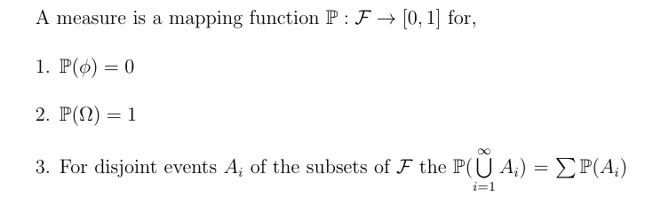
This is the actual definition of probability by the modern probability theory. After identifying these rules we can go on deriving other inferences. Now that we have formalized the actual definition of probability, we can actually move on to the cream of this article.

Let’s talk a little bit about discrete probability spaces.

Assigning probability measures on discrete probability spaces is quite simple, for example, we will look at two cases, one of finite Ω and the other of countably infinite Ω.

Borel Sets and Modern Probability Theory

But for uncountable Ω, it’s not as simple. So the classical example of an uncountable set is the interval of [0,1], which hs infinitely many points within it. Also, it was proved by Cantor’s Theorem that the cardinality of the elements between 0,1 is much greater than the number of natural numbers. This is the reason why we cannot assign a probability measure to singleton, as it will always tend to zero, and even if we want the probability of [1/2,1] that’s impossible too as we can only take union under a countable set.

So as to define a uniform probability measure over [0,1], we just assign probabilities to the subsets of Ω we find interesting instead of assigning probabilities to singletons.

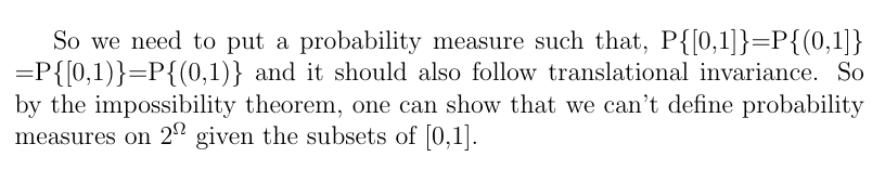
So as stated through impossibility theorem, we need to somehow shorten our sigma-algebra, so as to define probability measure on an uncountable Ω. We do this by assigning a probability to the sub-intervals of [0,1] which can be closed, open, open-closed, etc but this won’t form a sigma-algebra as it wouldn't be closed under complementation.

So now our goal is to generate a sigma-algebra, that contains the intervals we are interested in and is the smallest possible sigma-algebra. So,sigma-algebra containing all open intervals is termed as Borel Sigma Algebra and the elements of algebra are called Borel Sets. We can prove that Borel Sigma Algebra is the smallest possible algebra containing the sets we want. Hence Borel sets and Borel sigma-algebra have extreme utility when it comes to uncountable sample space.

Conclusions

1. Probability theory is a special case of measure theory
2. Probability is a function that projects events onto a number line