Principal Component Analysis: The Basics of Dimensionality Reduction

In the era of big data, we frequently find ourselves manipulating high-dimensional data, whether it be image data (where the number of dimensions will equal the number of pixels per image), or text data (where the number of dimensions is each unique word in a body of text) to name a few. Many times, it is desirable to reduce the dimensionality of this data since it can be represented accurately in lower-dimensional space. This can be useful for:

• data visualization (reduce to 2 or 3 dimensions so it can be graphed)
• minimizing the amount of data to a smaller size that still can hold meaningful information for more efficient storage or transmission
• data compression
• preprocessing information by removing portions of data that are highly correlated with other portions of data and are therefore redundant

So how do we do it?

Pure Intuition

We want to reduce the number of dimensions that are used to represent our data while maintaining as much information as possible. Before we start talking about how we go about doing this, let’s imagine ourselves in a similar, greatly simplified situation. Imagine there are two buildings in front of us. Our goal is to place the sun in a location that will best illustrate the differences of the buildings by the 2-dimensional shadows they project onto the ground. If the buildings differed only in height and we placed the sun directly above the two buildings, the shadows would lose all data that differentiated the two buildings and would look identical. If we put the sun 60° from the zenith, the 2D projection of the buildings will now show the difference in height.

Now imagine our buildings have similar heights and widths but different lengths; we would want to project the shadow onto 2 dimensions in the direction of the greatest difference between the two buildings, or else our shadows would not do a good job and distinguishing the difference between the two:

Similarly, we want to reduce the dimensionality of our data in a way that maintains as much information as possible. The end goal might be that we can restore the reduced data to something close to the original dataset, or perhaps we want to process the reduced-dimensionality data and achieve similar (or better) results than if we were manipulating the entire original dataset. So, we want to get rid of highly correlated, redundant data while maintaining the information that makes the samples unique, and we want to prioritize maintaining the information which has the largest “spread” of data, just like we wanted to project the shadows in a way that they would capture the differences of the buildings.

Let’s try exercising this idea with something closer to what we would be using Principal Component Analysis (PCA) for: imagine that we are working with image data, where every dimension of the original data is a certain pixel location in a given image. When we reduce the dimensionality, each dimension no longer represents a single-pixel location. Since we are losing this explicit, detailed information of each pixel’s exact value per location on a particular image, we want to focus on maintaining information about how the images DIFFER significantly. So, if there is a grouping of pixels that are always a certain value for those pixel locations in every single picture in our set, this information will not be useful for us to distinguish the differences between the pictures because it is the same for all of them. It is therefore not very important information to maintain in our reduced dimensionality representation of this set of images. Instead, we would rather focus on representing a series of pixels where there is a significant difference in shade between the pictures, because then our reduced-dimensionality data will still hold the information that makes our images distinct, and thus our images will be sufficiently different from each other in a reduced-dimension representation. This is similar to putting the sun behind the area of the buildings that were the most different. These directions with the largest spread (or variance) of data are called the principal components of the data.

Mathematical Intuition

To ensure that we are not keeping redundant data, we want our new reduced dimensions to be uncorrelated, so we need to make sure they are orthogonal (e.g. exist perpendicular to each other). Also, if we are reducing from N number of dimensions to a reduced R number of dimensions, we want to prioritize directions that have the largest variance of data, as described above. It is important to note as well that these new dimensions in our reduced dataset will not be the same dimensions that existed in the original dataset. This is important because a side effect of PCA is that there is less intuitive meaning to the dimensions we end up with than the ones we started with. For example in the original data, one dimension might mean the 5th pixel in the first row of an image or the word “computer” in a body of text, but in a PCA-manipulated dataset, one dimension would not have the same intuitive meaning, because it was derived mathematically in a way to maintain as much information as possible.

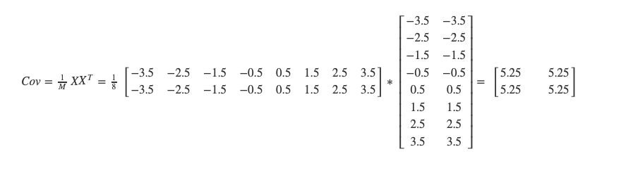
To find sets of orthogonal vectors that describe the principal components of our dataset, we can use eigenvector decomposition of the covariance matrix of our data. The covariance matrix will simply be a square matrix that shows the covariance between the different dimensions of our data, and it is calculated by multiplying our centered data matrix by its transpose with a multiplied scaling factor.

Eigenvectors describe a vector that, when multiplied by the dataset it was derived from (in this case our covariance matrix), yields simply itself (that same eigenvector) scaled by a certain value (called the eigenvalue of that eigenvector):

This is significant because these eigenvectors describe an orthogonal (uncorrelated) set of vectors which delineate the principal components of our data, and the magnitude of the eigenvalues will describe which of these eigenvectors correspond to large variances of the data in that direction, and therefore the dimensions we want to choose for our PCA representation. Finally, we take our (centered) original data and project it upon these eigenvectors with large eigenvalues to create our new reduced-dimensionality data.

Let’s do a few examples, and start with something extremely simple to get some comfortability. A perfectly correlated 2-dimensional dataset should be able to be turned into a 1-dimensional dataset with no data lost, and with easy visualization of what we want to do.

Let’s say this is our data:

s1 = [1,2,3,4,5,6,7,8]
s2 = [1,2,3,4,5,6,7,8]

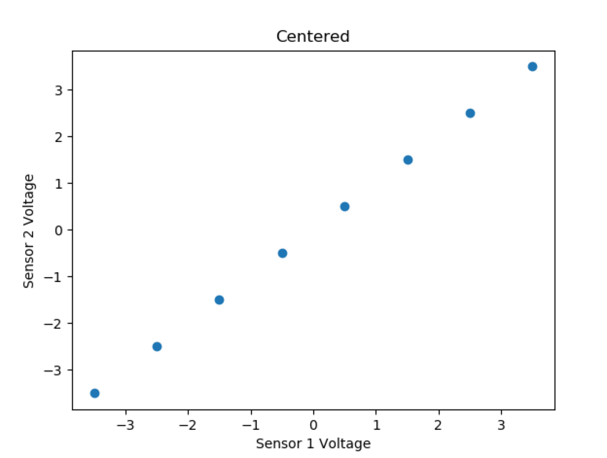
To put some meaning to these numbers, we have two sensors, s1 and s2, sensing some input parameter and outputting voltages for us to read. We can say each s1,s2 output pair occurs at some point in time different than another s1,s2 output pair. It should be intuitive that we can represent this information in 1 dimension, because each s1,s2 output pair is identical and perfectly correlated to each other. Let’s follow the intuition we presented above to do this.

Here is our collected sensor data:

First, we said we wanted to center our data, and then create a covariance matrix. Let’s start by combining our sensor data pairs into a matrix X:

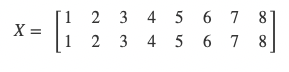
Notice we made the data matrix X an NxM matrix, where N is the number of dimensions (2) and M is the number of data points per dimension (8).

Now, we will center each dimension’s data around 0:

And calculate the covariance matrix:

Now, we calculate the eigenvectors and eigenvalues of the covariance matrix. You can do that using the equations:

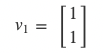
Or, since we are working with a symmetric square matrix in this sample case, you can do so by inspection:

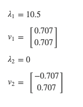
Eigenvalue 1 is the sum of the rows: 5.25 * 2 = 10.5
The sum of the eigenvalues is the trace of the matrix, so eigenvalue 2 = 10.5–10.5 = 0

Since the covariance of s1s1 to s1s2 is the same as s1s2 to s2s2, the eigenvector associated with the eigenvalue which is the sum of the rows is:

The second eigenvector must be orthogonal to the first:

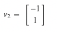
Then, normalize the vectors to get:

You can calculate these quickly in python using the numpy library:

import numpy as np
cov_mat = np.matrix(your_data)
d,v = np.linalg.eig(cov_mat)

Or ruby:

require ‘matrix’
cov_mat = Matrix[your_data]
eig = cov_mat.eigen
d,v = eig.d, eig.v

To quickly calculate in ruby, you will want to use a library which is faster (see code below). Using GSL::Matrix yielded the best results for me with minimal setup.

No matter how you do it, you end up with the eigenvectors and associated eigenvalues above. Now, since we want to go from 2 dimensions to 1 dimension, we use the eigenvector associated with the larger eigenvalue to reduce the dimensionality. Just like our buildings, we are projecting our data points on the eigenvector. In this simple case, it turns out that all of our points are all on the eigenvector itself:

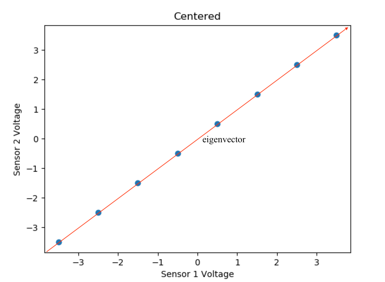
This projection corresponds to multiplying our eigenvector as a single row matrix (dimensions 1x2) by the centered data (dimensions 2x8), resulting in the 1-dimensional dataset (dimensions 1x8):

[-4.95, -3.54, -2.1, -0.707, 0.707, 2.12, 3.54, 4.95]

Which perfectly describes our data, but no longer corresponds to individual sensor outputs.

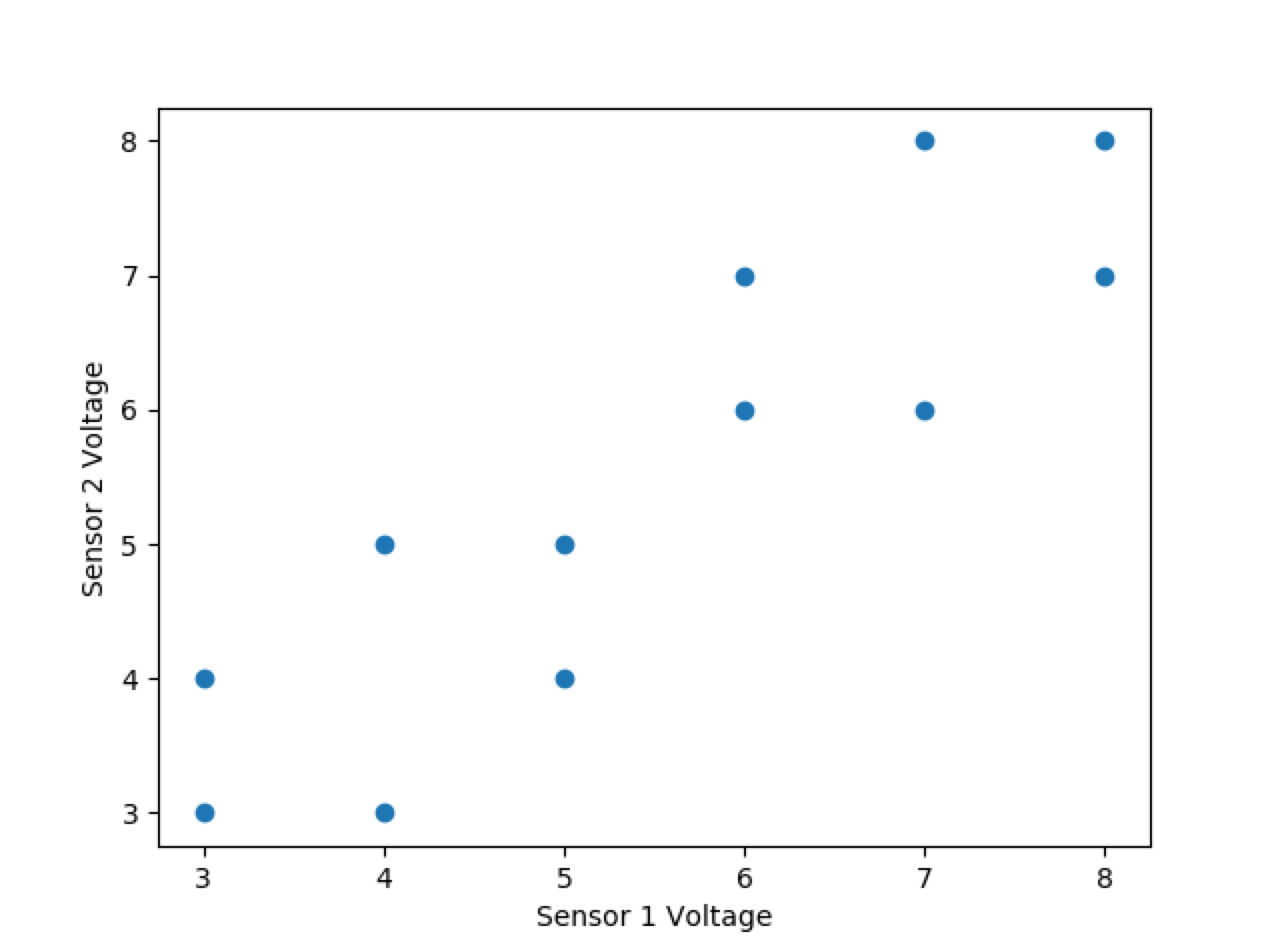
Let’s quickly look at a slightly more complex 2-dimensional example, where now the data points do not all lie on the eigenvector and must be projected with some data loss:

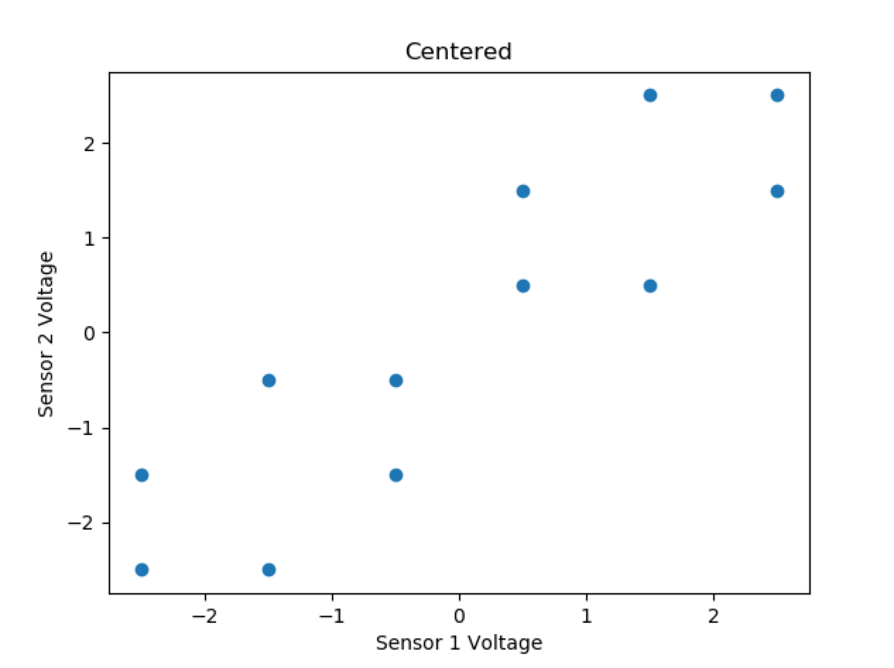
x = [3,3,4,4,5,5,6,6,7,7,8,8]
y = [3,4,3,5,4,5,6,7,6,8,7,8]

Centered Data:
x = [-2.5,-2.5,-1.5,-1.5,-0.5,-0.5,0.5,0.5,1.5,1.5,2.5,2.5]
y = [-2.5,-1.5,-2.5,-0.5,-1.5,-0.5,0.5,1.5,0.5,2.5,1.5,2.5]

Covariance matrix:

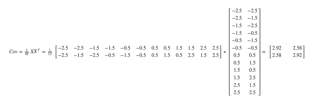
Covariance matrix eigenvalue decomposition:

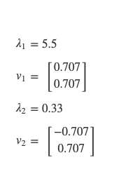
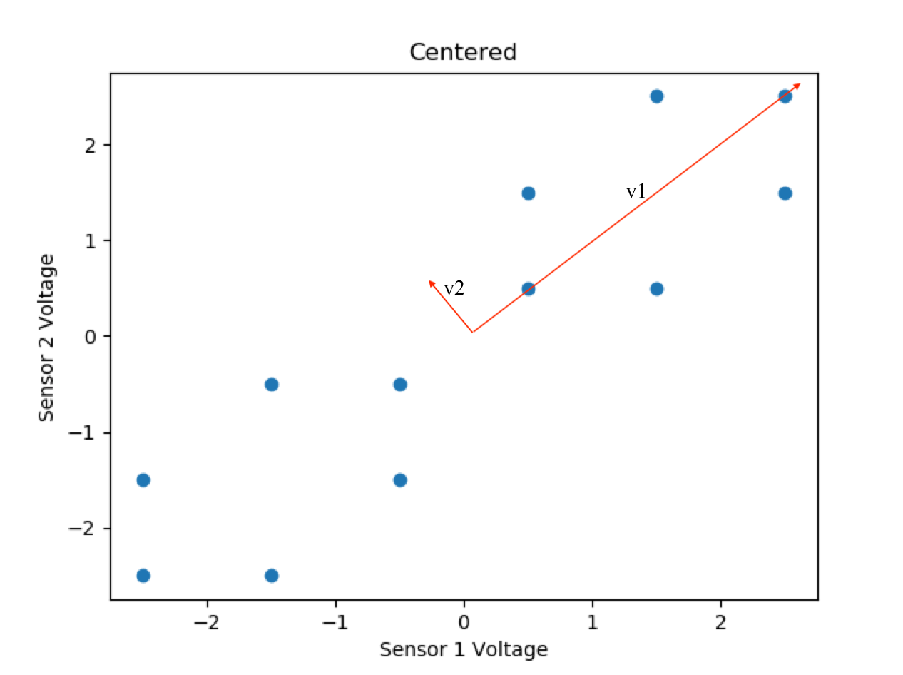
Again we choose v1 as our eigenvector with the greatest variance in data because it has the larger corresponding eigenvalue, but this time all of our points do not lie on it. So, our 1-dimensional representation will be projections of those points on our single eigenvector. Notice that due to the symmetry of the points, there are several sets of 2 points which project to the same point on our 1-dimensional line.

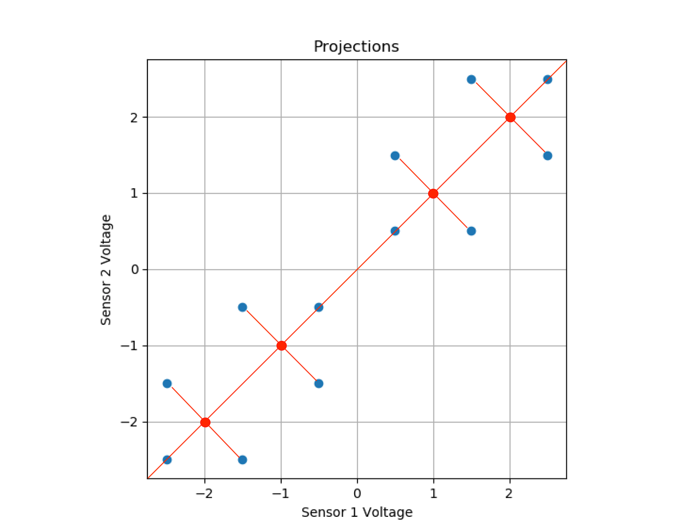
Giving the 1-dimensional points:

[-3.54, -2.83, -2.83, -1.41, -1.41, -0.707, 0.707, 1.41, 1.41, 2.83, 2.83, 3.54]

Clearly, data has been lost in this transformation to 1 dimension, because there were multiple points perpendicular to the main eigenvector that shared a projected value. Notice, however, that more information was maintained than if we had just chosen one of the original dimensions to maintain, where we would have lost half our data.

Mathematics

In the intuition portion, we jumped to the conclusion that eigenvectors of the covariance matrix will give us the dimensions which retain the most data. Let’s confirm that with some math.

First, let’s mathematically define what we want. We want to find a matrix of orthogonal normalized columns (U) that we can project our (mean-centered) original data (X) onto that will retain as much information as possible from our original dataset, but represent it in a reduced number of dimensions, R. It is important to note that this matrix U will be the tool we use to perform the dimensionality reduction and reconstruction processes. The U matrix has the shape NxR, where N is the number of dimensions of our original data X (whose shape is NxM as described below), and R is the number of dimensions to which we want to reduce the data. Thus, UU_transpose, aka P, has dimensions NxN.

The input data X has dimensions NxM, so we project this data upon a reduced dimension set of vectors with the product reduced = U_transpose * X, and restore to an approximation of X by restored = U * reduced . If we were to do this in one step, it would be U * U_transpose * X . Remember that for the discussion below.

PCA is completely defined by the solution to the following equation:

Where:

• F is the Frobenius Norm (which is like the Euclidean Norm, except for matrices)
• Pk is a set of orthogonal projection matrices P, each of which is idempotent (P² = PP = P), orthogonal (P * P_transpose = I; and so P_transpose = P_inverse), and is the product of UU_transpose where U is a matrix which contains orthogonal columns as described above.
• X is the mean-centered NxM input data matrix (e.g. each point centered relative to the mean of its dimension)

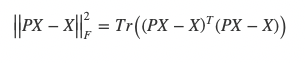
Remember our description of the reduction and restoration process above. This equation now makes sense because P is U * U_transpose, where U is comprised of normalized orthogonal columns. So, P * X is equal to U * U_transpose * X, in which U_transpose * X projects X onto the (reduced number of) orthogonal dimensions, and U * U_transpose * X restores a prediction of what X originally was from the reduced state it was in. So, P * X is an approximation of X based on the reduced-dimension form, and we want to minimize the error of the original dataset X with the reduced and restored version of X, which isP * X. To reduce this error, we reduce the Frobenius norm of the difference of the full-dimensioned data and its reduced and restored approximation as the equation above describes.

The definition of the Frobenius Norm is:

Where Tr(-) is the trace of a square matrix, i.e. the sum of the diagonal values starting at (0,0) to (N,N) for a NxN matrix.

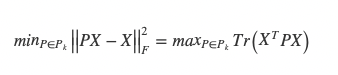
So, we can write the problem now as:

Which, taking advantage of the fact that P is idempotent and the property of linearity, reduces to:

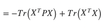
And since Tr(X_transpose * X) does not change with respect to P, our new problem is:

Since P=UU_transpose, and a trace is invariant under cyclic permutations, and U is made up of orthogonal columns, our problem becomes:

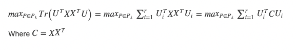
To solve this summation, since the columns of U are orthogonal, we want to maximize U_transpose * C * U with respect to some restraint on the size of U_transpose * U , so we do not achieve a maximum simply by making U large. To find the max based on this restraint, we can use Lagrange, and make the restraint that U_transpose * U is of unit size:

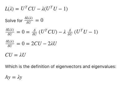
So mathematically we now come to the same conclusion as in our intuition — use the eigenvectors of the covariance matrix (which is just a scaled version of our matrix C = X * X_transpose above, and will, therefore, have the same eigenvectors just with proportionally scaled eigenvectors) to create the lower-dimensional representation of our data with the least amount of reconstruction error.

(TLDR Start) Algorithm

Input: X= [x1, …, xM] where each xi is a row of size N, where N is the number of dimensions and xn is an array of all data in that dimension. So really, Xis an NxM matrix, where N is the number of dimensions and M is the number of datasets in those dimensions. For example, if we have 100 images with 400 pixels each, N will be 400, and M will be 100. x1 will be an array of 100 numbers, the first pixel of each image. xM will be an array of the 100 values of the 400th pixel in each image.

1. Center the input data by subtracting the mean of each row from each element in that row. For example, subtract the mean value of all pictures’ first pixels from each first pixel value. Do this for each pixel. Now, instead of pixel values being from 0–255, they will be centered around 0.

2. Calculate the covariance matrix C, and then its eigenvectors and eigenvalues. As described previously, the eigenvectors of the covariance matrix will be the same as the eigenvectors of the original data, and the eigenvalues will simply be scaled:

3. Create a new matrix V made up of the R eigenvectors associated with the R largest eigenvalues stacked vertically in descending order of their corresponding eigenvalue, where R is the number of reduced dimensions. This matrix U will be of dimensions MxR

4. Calculate the reduced-dimension representation of the data as the matrix Y of dimensions RxM:

The matrix Y is the reduced-dimension representation of the centered version of the original data.

To reconstruct an approximation to the original data, just multiply Y by the R eigenvectors used to reduce the data (not transposed), and then add the original row mean back to every element:

and then simply restore each row’s average back to every element in that row.

Code

I have written out the logic in Ruby because Python has plenty of libraries that allow you to perform PCA. Note that I use the GSL library for matrix operations because the standard Matrix implementation built into ruby is much too slow for efficient calculations, but I try to return stdlib Matrix objects to the user of the code as much as possible.

Practical Usage (MNIST Database)

Note that in the code below, the PCA class is namespaced under the module Rbmach. That is the gem it will be published in, and you can use it or contribute if you wish once it is released! I also use another little gem I write called Rbimg which allows you to create a png image using an array of pixel values. (It will also let you read png images as an array of pixel values).

Here I am reading 1000 images from the MNIST database of handwritten numbers. Each image is 28x28 pixels long, which means that each image has 784 dimensions. I reduce the set of 1000 images to 2 dimensions per picture up to 322 dimensions per picture in steps of 10 and graph the error of each reduced representation once it is restored. I also use the pixels from the restored version of the pictures to show visually what the image would look like after being reduced and restored. Note that a restored image will contain as much information as its reduced source.

As you can see, the errors are quite high with the original 784 dimensions shown in only 2 dimensions per picture, but it quickly reduces significantly to less than 2% with significantly fewer dimensions than 784.

Let’s take a look at a full-dimensionality image, and then what some of the reconstructed images look like, and what their data looked like in their reduced form.

Here is one of the original images with a dimensionality of 784 pixels:

Now let’s look at the same image reconstructed from 2, 12, 22, 32, 42, and 272 dimensions against the original 784-dimensional image:

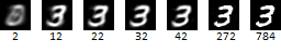
We can see that the images are recognizable with significantly fewer dimensions than the full 784. At 22 dimensions, our image is quite clear when restored, and instead of 784 data points, our handwritten 3 is represented as such:

[-518.0, 592.6, -87.5, 887.5, 111.4, 977.0, -346.5, -208.1, -11.6, 144.5, 62.2, 60.5, -162.3, -125.0, -111.6, -17.1, 313.7, -279.7, 45.3, -116.6, 26.0, -157.6]

Depending on your application, you can use significantly less data to perform your calculations. For example, let’s show 4 different images restored after being reduced to 22 dimensions:

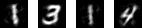
The numbers are 1314, where the two 1s are different drawings of a 1. Not only are these images recognizable to the human eye, but we can quickly demonstrate that their reduced form of just 22 dimensions per image holds enough information to perform non-trivial operations on them. In the below example, I use a non-supervised learning algorithm (K-means) to cluster these 4 images into 3 “groups”. The successful grouping of the two images of a 1 into the same centroid consistently with the 3 and the 4 being assigned to two different “groups” is a good fast showcase of the fact that there is enough information stored in 22 dimensions to perform a relatively successful unsupervised learning algorithm on the data, which will be much faster with 12 dimensions than with 784:

P.S. There are ways to use apply the kernel trick to PCA in a similar way that it is used in Support Vector Machines. I will write a piece on it after exploring it in the context of SVMs. Until then, happy PCAing!