Numerical Solvers for ODEs

This story will give you a brief introduction to the basics of numerical integration and how it is used to solve Ordinary Differential Equations. I will cover the explicit Euler and implicit Euler method as well as Heun’s method in this story.

1. How to solve ODEs numerically
2. Explicit Euler
3. Implicit Euler
4. The combination of both Euler methods (aka Heun’s method)

How to solve ODEs numerically

Ordinary Differential Equations are not only a special set of equations in mathematics. From the perspective of an ongoing engineer, ODEs can be used to describe dynamic systems in our real world. So let’s go with an example.

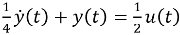
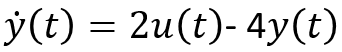
Equation 1 shows an ODE of a PT1-System. This could be e.g. a simple RC-low-pass filter. The analytical solution is:

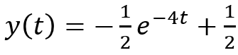
In this case it it quite easy to solve the ODE analytically, but if things get more complicated and an analytical solution is not the way to go, we can solve ODEs numerically. To be more precise: We can approximate the solution.

I won’t go deep into the details here, but the idea is to calculate the gradient at a given point and then approximate a solution (y) at the next point by using this gradient and defined increment. As we decrease the increment we increase the accuracy of our approximation but it takes more computational power to solve the ODE. To calculate the gradient we just have to rearrange Equation 1 and get:

Now we can calculate the gradient at any given time if we know the current value of y and the time (we assume that u is constant over time). In most cases we have given starting conditions where we know the gradient and the value of y. From this starting point on we have everything to approximate our solution.

Explicit Euler

The explicit Euler method is the most simple way to perform the approximation.

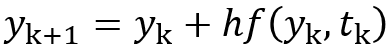
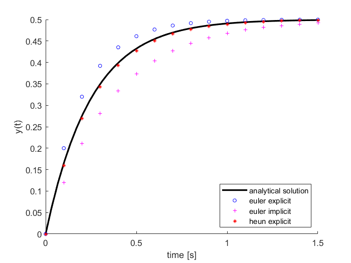
The approximation in the k+1-th increment (or step) is calculated by adding the product of the increment h and the gradient f to the current solution. As described before, the gradient is a function of the current value of y and the time. It is assumed that the gradient is constant over time. Figure 1 shows how this affects the solution. The explicit Euler “reacts” too slow and overshoots in this example.

Implicit Euler

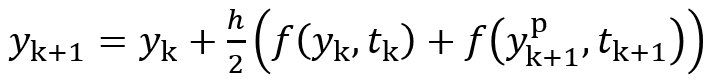
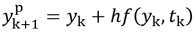
The implicit Euler uses 2 explicit Eulers to approximate the solution. The first is called the “predictor” and second is called the “corrector”. The approximation of the predictor is used to approximate the solution again with an explicit Euler.

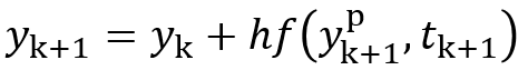
The corrector-approximation tries to correct the predictor-approximation by calculating the gradient at the predicted point instead of the current one. This tends to create the opposite behavior as observed before (Figure 1).

Modified explicit Euler method (aka Heun’s method)

Heun’s method combines both explicit and implicit Euler methods by averaging them. Figure 1 clearly shows how the error of both Euler methods are cancelling out each other.