Before we begin, be aware that talking about control theory in any meaningful way means talking about linear algebra. Please don’t be intimidated, even if you don’t have the first idea what any of the symbols or terms mean. Linear Algebra is hard but its core ideas are intuitive and I will explain everything as we go.

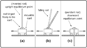
In the first article, we explored the world of control systems. We saw how control systems are present all around us for ages and how it makes our life safe and easy. The problem “control of an inverted pendulum” was proposed to understand various control strategies and concepts. Refer this article for insight into the inverted pendulum.

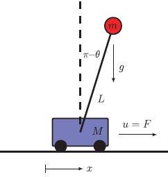
For this study, I will be placing the inverted pendulum on a cart with a friction-less base. The connection between the pendulum rod of length L (assumed weightless) and the cart has damping (d). Damping is the resistance towards change in angular speed of the rod. The figure below shows the setup:

I will not go through the derivations of the equation. That is something we can find anywhere easily. It is also well understood with a video rather a textbook derivation. On the other hand, to understand the analysis of the equation one needs the understanding of state variables and equilibrium points. 
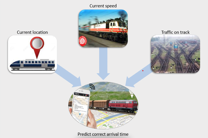
State variables are the minimum number of variables with which we can completely define a system. Too formal? Don’t worry. Take, for example, the train for which you are waiting on the platform. You look into your train tracking app to get an idea when it will arrive. Which information is needed by the app to correctly predict the arrival time of the train? Well, its current position, its speed and the traffic on the track will be used to correctly predict the arrival time. So, look back on the definition and you will find that the current position, the current speed and the traffic are the state variables here.

If you express this in terms of equations and mathematical model then the whole expression is called state-space expression.

Now, the equilibrium points. Put all the derivative of the state variables to zero you will get the equilibrium point. Basically, in the equilibrium point, there is no change in the state variables with respect to time. Hence, the rate of change is zero. So, when the train arrives at the platforms and stops, you get the equilibrium point.

Mathematical Modelling

The equation for the inverted pendulum is given below. You can see how the equation are written in terms of state variables, which are, the position of the cart {x}, its speed {v}, the angle which the ball pendulum makes with the vertical {θ} and its angular velocity {ω}. So, the state vector X = [x, v, θ, ω]’, where “ ‘ ” denotes the transpose.

These are the differential equations (equations which describe a rule for the rate of change of a function with respect to one or more of its input variables). The dot “ . ” on the top of state variables means their rate of change with respect to time. 
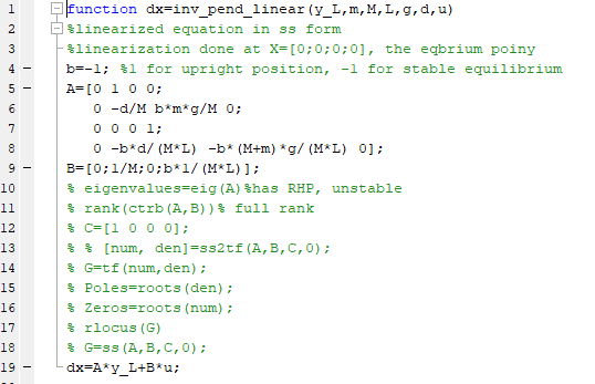
Mathematical models can be well coded in MATLAB. MATLAB is an engineering-specific programing language, helps us to write the mathematical models easily. Check the simple code of the above equations below. To view all the MATLAB codes related to this series, go to this link of GitHub.

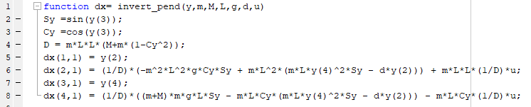
Above, dx is the time derivative of the state vector X.

If you find the equilibrium point here by equating all the above equations to zero, you will get two points. These two points, corresponding to either the pendulum down (θ = 0) or pendulum up (θ = π) configuration; in both cases, v = ω = 0. The upwards position is an unstable equilibrium point. The downward position is stable. We will later see how we can identify different the equilibrium points using simple math. A disturbed pendulum will always go to the stable position unless a control force is applied (see the videos below). 
From here onward, the complete setup of the pendulum and the cart will be called the system.

Developing the linear model

Looking at the equation above, we see that terms like sin(θ), cos(θ), ω² make the system non-linear. They pose a problem in designing the block-diagram or representing in a neat constant matrix of a state-space format or transfer function format. Hence, modelling and analysis become difficult. Also, many linear control techniques are available like PID, LQR (we will discuss them when we design the controller) and they are easy and tried-and-tested methods to deals with linear systems.

So, we try to develop a linear model of this system using a process called linearization. For linearization, we need an operating point as explained in the appendix. The equilibrium point is an operating point. But we have two equilibrium point. Hence, the linearized expression depends upon which point is chosen. The linearized matrices look like this as shown below

where b=1 for the pendulum upward equilibrium point, and b=-1 for the pendulum downward equilibrium point. The above expression can be simply written as

We call A as the state matrix, B as the input matrix, C as the output matrix and D as the direct output matrix. Y is the output matrix. Look how clean and easy the above expression is when compared to the non-linear dynamics. The uncontrolled system performance depends upon A matrix. The code looks like this

Analysis of the linear equations

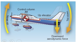
Before proceeding, let us revisit the stick on the finger analogy from the second article. As mentioned there, to move the stick forward, you first need to pull the finger back, giving a forward tilt and then move forwards. This type of system where the physics of the system forces it to dip/move in the wrong direction initially to achieve its correct direction is called “non-minimum phase system”. Other examples include the altitude manoeuvre in aircraft and parallel parking.

Non-minimum phase systems can easily be identified from their transfer function. The presence of a right-hand side (RHS) zero makes it a non-minimum phase system. The transfer function (output/input) of the system is shown below:

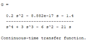
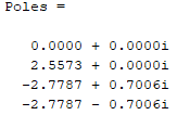
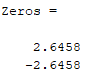
One of the roots of the numerator of G(s) i.e. zeros is positive (+2.9458) is a result of the system being a non-minimum phase system. Zeros only chance the amplitude (except the RHS zeros) of the response, not the overall characteristic. 
Here we can see that the system has an RHS pole. RHS pole leads to positive exponential terms like e^t, which leads to an unstable response.
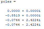
When the model is solved with b=-1, we see that all the poles of the system are negative (LHS) and the response is stable. Hence, when simulated with b=-1, we get stable dynamics as shown below in the simulation section.

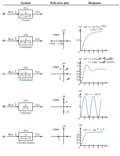
The poles of the transfer function are what majorly defines the response of the system. Depending upon the placement of the poles the system can have a fast response or slow response. This is measured using defining characteristics like rising time, settling time, peak time, percentage overshoots etc. So, if we change the pole location, we can change the performance. This is the motivation behind the pole placement technique in the control system. Refer the image below to see the change in response. It is less intuitive than the classical methods like PID controllers but is easily understood and implemented.

Simulations

To make it intuitive, I have written another code to represent the motion of the system in a video. It is shown below. You can see how it goes down, to its stable equilibrium point without any control force. This is the non-linear dynamics

The linearized system dynamics around the unstable equilibrium point (b=1) is shown below. we can see how it overshoots and behaves erratically.

Check the video below to see how the system behaves when simulated with b=-1 i.e. unstable equilibrium. You can see the difference, it behaves similar to the non-linear dynamics.

We will develop various control techniques to control the inverted pendulum in the later series of articles. But before that we will learn about the crown prince of the modern control technique — The concept of controlability and observability in the next article.

Appendix

Linearisation

This is a mathematical process that helps us find linear approximate to a function at a point. This point is called an operating point and the approximation is valid about his point only. An operating point can be any point from where the trajectory of the system passes i.e. any point which is the solution to the equations which define the system. It is done through the Taylor series expansion of the function about the operation point and neglecting the higher-order terms (HOTs, terms with the power of x greater than 1)

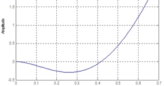
Take the example of a function y=f(x)=x². Applying the Taylor series expansion about x0=2 and neglecting HOTs we get the following linear equation:

f_linear(x)= 2²+2*2(x-2) = 4+4(x-2) = 4x-4

The plot of non-linear and linear equation are shown below:

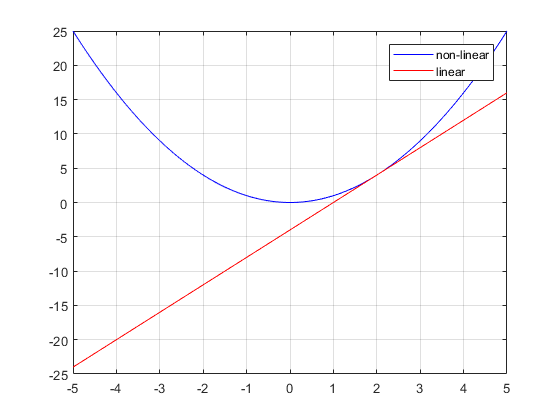
Notice that the linear equation represents non-linear equation only around x=2 i.e. the operating point. This is an important consideration when designing a controller based on linear model — it is only valid for small inputs about the operating point.