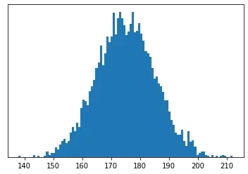
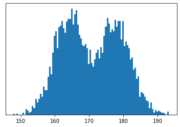
Suppose, as we all do on a Friday evening, you are looking at data of all the heights of people attending a university. You can plot a histogram of all the data and it might look something like this:

You hear that there will be a new person arriving tomorrow and you want to find out what the probability that their height is within 5 cm of yours. How do you go about doing this?

1. Guess the Shape

The first thing we want to do is to construct a probability distribution that best ‘fits’ the data. In order to do that we have to decide what sort of distribution we are dealing with.

Gaussian seems like a reasonable guess.

For a Gaussian, we need two parameters, the mean μ and variance σ². We could just use the boring estimates by finding the average and standard deviation of the data but where is the fun in that! Instead we are going to use a much more general tool called maximum likelihood estimate.

2. Compute the Likelihood

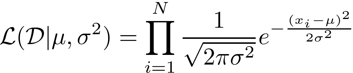
Assume that our height data has been sampled independently from the same Gaussian distribution (our data is said to be i.i.d — independent and identically distributed). We can determine the probability of seeing that data given some mean and variance. Call L the likelihood of seeing our dataset D = {x_1, x_2, …, x_N} and by exploiting the fact that each sample is independent and so can be written as a product:

We now want to find the mean and variance that gives us the largest likelihood of observing this data. That is we want to find

Solving this is quite hard, so instead we are going to use a nifty observation. Suppose we have some function f and we want to find argmax f(x), then for any monotone (decreasing) h, we have argmax f(x) = argmax h(f(x)). (If h is monotone decreasing then the argmax gets swapped to argmin.)

Notice that log is a monotonic increasing function. So we can write:

This is referred to in literature as the log-likelihood of the data. Jumping a few tedious steps (left as an exercise to the reader!) we can see that the log-likelihood is:

3. Solve for Optimal Mean and Variance

We now want to find the largest value of this by picking the optimal μ and σ². That is simply a case of finding the derivatives and setting them to 0!

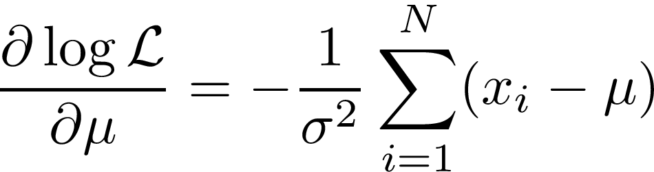
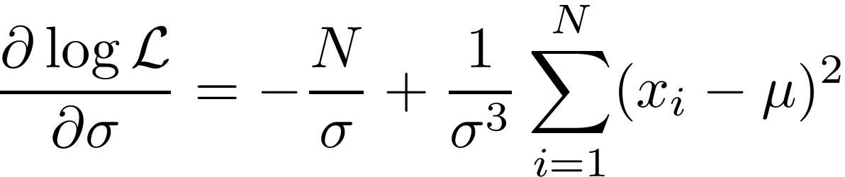
Solving these for 0, we get the following (and very familiar) equations:

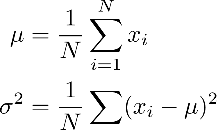
So we have just done a very roundabout way of showing that indeed the mean and (biased) variance estimates are indeed the correct choice of parameters.

Conclusion

So what is the point of doing all this if all we are going to do is recover the equations for mean and variance we already knew?

Well this method can be applied in more complicated situations. What if your data now looks like this:

or what if your guess for the underlying model is something like this:

Where the free parameters are f and t_p.

In these cases, solving it with explicit equations is not going to work but attacking it with maximum likelihood estimate might just do the trick.

In the next article, I will discuss how to use maximum likelihood in a non trivial way to compute a distribution (or at least derive an algorithm to compute it) for some more complicated data.

Addendum

You might remember that at the start we wanted to know the probability that the newcomer’s height would be within 5 cm of mine.

The maximum likelihood estimate for the mean was 175.02 cm and variance was 99.66 cm² (the parameters I used to draw the data were mean of 175 and variance 100).

Then it is a simple case of integrating the probability distribution between my height-5 to my height+5:

I leave it as a secondary exercise to the (very) interested reader to figure out my height.