Maximum Likelihood Estimate

If you haven’t read part 1, you can find it here. The general gist of it is that we look at our data and have a guess at what sort of model would fit it best, then we find the parameters for that model that are the most likely to have generated our data.

As promised, we will look at something more complicated now.

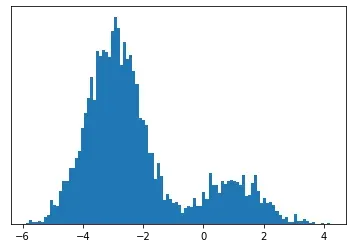
Consider the histogram of our data is the following:

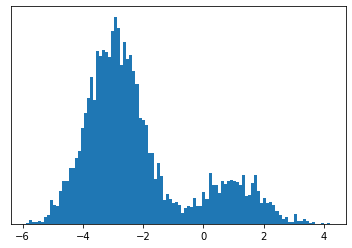
It doesn’t look like anything you will have encountered in high school statistics.

Well, sort of.

One could argue that it looks like two Gaussians mixed together.

To figure out what model to use, we can think about how this data was generated.

I propose the following ansatz model:

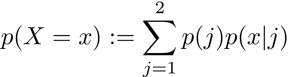
Where j is a Bernouilli variable.

Let us unwrap this equation. We have two Gaussians with means μ_1, μ_2 and variances σ²_1, σ²_2. The probability density function of these is given by p(x|j) where j can be 1 or 2. We have another random variable, j, that is a Bernouilli variable that acts as a mixing component.

To generate the data, simply sample the Bernouilli variable, this tells us which Gaussian to further sample from.

So when we are estimating our parameters, not only do we have to estimate the means and variances but we have an extra thing to calculate and that is which data point comes from which Gaussian. We wrap this up in an indicator variable called Z, defined as follows:

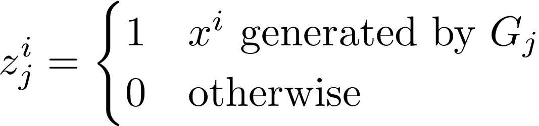
Where x^i is the i-th data point and G_j is the j-th Gaussian. Now we can write the probability of observing a data point is:

Z is a (latent) random variable so we can compute the expected value of it. We call this expected value the responsibility and can define it as follows:

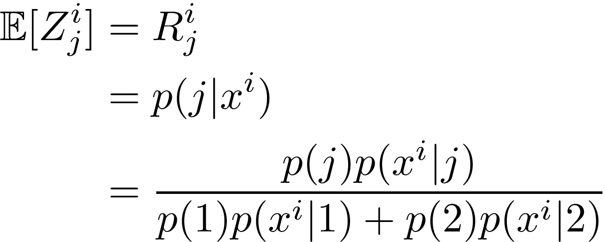
The last line follows by Bayes’ theorem.

We are now in a position to write down the likelihood of observing our data D. Recall that the likelihood is just the product of all the probabilities:

For technical reasons I won’t go into, instead of computing the log-likelihood like we did last time, we will compute the expected log-likelihood. I will leave it as an exercise to show that the following holds:

Now it is not so easy doing this by hand so instead we are going to optimise it via coordinate wise ascent. What this means in our case is that we will optimise the mean and variance parameters, then optimise the mixture coefficients p(j). Using these new parameters, we recompute the responsibilities, and repeat.

Step 1: Optimise Gaussian parameters

Note that the only term that is dependent on the Gaussians in the expected log-likelihood is T_2. So we can differentiate the expected log-likelihood with respect to μ_k and σ_k to find

Similar to the previous article, we set these to 0 to find the optima. (We would technically need to also look at the second derivative to make sure that we are finding a maxima but that is very finicky so will be omitted.)

We now get our maximum likelihood estimates (MLE) for mean and variance:

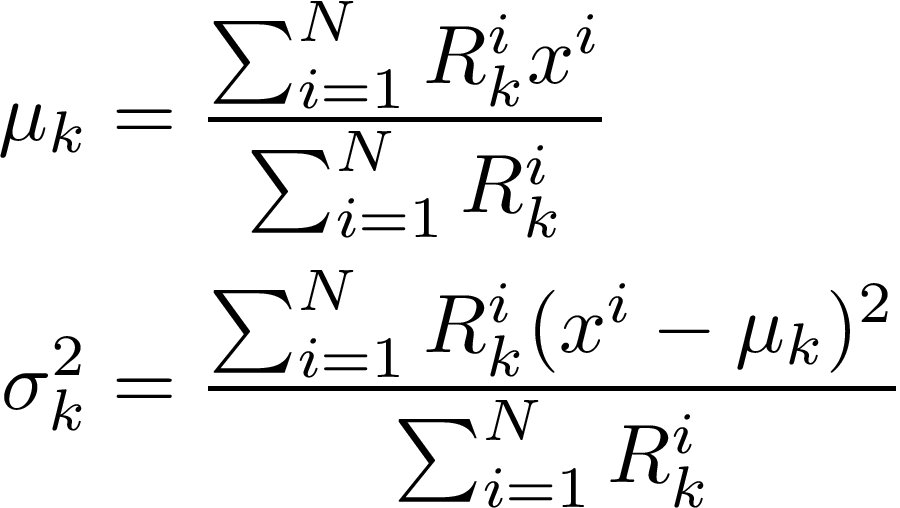
Intuitively, this is just the regular estimates that we derived in the previous part but each data point is weighted with how ‘responsible’ that Gaussian is for the point in question and then normalised. This can be seen by looking at the best case scenario: if we know exactly which point comes from which Gaussian, then the responsibility is either 0 or 1 and these equations collapse to exactly the regular maximum likelihood estimates of mean and variance.

Step 2: Optimise the mixture coefficients

Now we want to maximise our mixture coefficients. Recall that these are the probability of sampling from each Gaussian.

Similar to step 1, we note that T_1 is the only term that is dependent on the mixture coefficients. We could just do exactly what we did above — that is differentiate with respect to p(k) and set it to zero.

But when is math ever that simple?

Since the mixture coefficients form a probability distribution, we have an additional condition that p(1)+p(2) = 1. So we can’t just optimise willy-nilly, we have to include this constraint in the equation. This is exactly the kind of problem that Lagrange multipliers is useful for.

If you aren’t familiar with Lagrange multipliers, don’t worry I won’t dive into the derivation. If, on the other hand, you do know the method of Lagrange multipliers, I leave you to check the derivation yourself.

In any case, we get the new mixture coefficients:

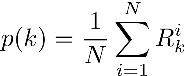
Again, this makes sense if you interpret it as the average number of points each Gaussian is responsible for.

Step 3: Recompute Responsibilities

Now that we have optimised the parameters of the model, we can recompute the responsibilities.

This can be done using the Bayesian expansion from the definition of responsibility.

OK great so we have this theoretical framework, now to apply it to our data.

We randomly initialise the means, variances, and mixture coefficients. The means and variances have to be somewhat close to the true value or else the algorithm will struggle to converge.

Then from that we can compute the responsibilities.

Using these responsibilities, we can recompute the parameters via the regime described above.

This process will converge to the true model. Below are some snapshots of the converging process

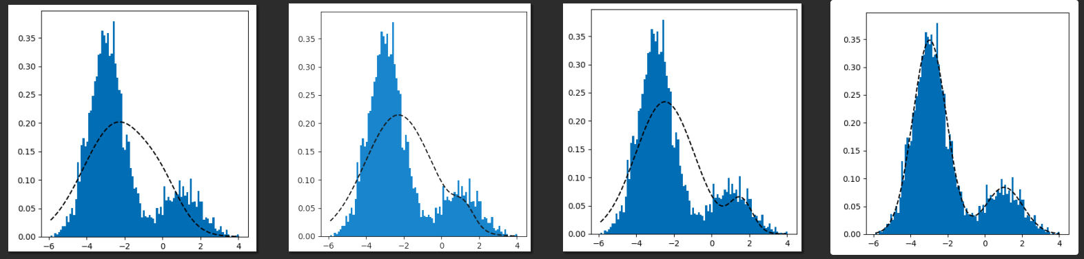
This can be extended to multiple Gaussians and is not restricted to Gaussians at all.

Consider for example a shop owner who wants to model the number of customers that walk into their shop throughout the day. A sensible base model would be a Poisson distribution. However, we can expect that the mean number of visitors in the shop will vary throughout the day — for example it could be busier at lunch time and then again in the evening. So a mixture model of Poisson variables would be appropriate.

I will leave it as an exercise to derive the update equation for the parameter of the Poisson. As a few hints:

The expected log likelihood equation holds, you just need to change the value of the distribution. The equation for the mixture coefficients are model independent.