If you’re unfamiliar with Stochastic processes, then I would suggest that you read my introductory article on the topic, as it covers all the background needed to understand this next tutorial. If you’re already familiar with the topic, please read on.

This tutorial focuses on using matrices to model multiple, interrelated probabilistic events. As you read this article, will learn how calculate the expected number of visits, time to reach, and probability of reaching states in a Markov chain, and a thorough mathematical explanation of the application of these techniques.

Three Heads in a Row 💰

Let’s start with a simple probability question:

Q: What is the expected number of tosses to get 3 heads in a row with a fair coin?

You can solve this using prior knowledge of probability and geometric series but using a Markov chain will give you the answer to this question and more, in a way that is not only quick, but also generalizable to other problems with the same basic idea that are much messier than this one. Let’s start by constructing a transition probability matrix for this question:

coins <- cbind(c(.5, .5, .5, 0), c(.5, 0, 0, 0), c(0, .5, 0, 0), c(0, 0, .5, 1))
dimnames(coins) <- list(c("_","H","HH","HHH"), c("_", "H", "HH", "HHH"))coins
_ H HH HHH
_ 0.5 0.5 0.0 0.0
H 0.5 0.0 0.5 0.0
HH 0.5 0.0 0.0 0.5
HHH 0.0 0.0 0.0 1.0

At each step, we see there’s a 50 percent chance to go to state 0, a 50 percent chance to move to the next state, and an absorbing boundary at state 3, where our criteria for stopping is met.

What are we trying to find right now in terms of the matrix that’s currently in front of us? Well, if we had an expected number of visits to each individual state at every step, then we could just add those up to get the total number of times we visit a state before absorption. Let’s start in state 0 and try to think of a way to estimate how many times we’ll visit there. For the first step, we expect to visit state 0 50% of the time, so that is half a visit. If we take another step, then that’s just M²(0, 0), which is .5, and then M³(0, 0) =.5. In theory, if we continued to sum these numbers for every positive power of M, we would have the total number of expected visits. (“But wait!”, I hear you shout at your computer, “What if the sum diverges!?” Excellent question. Recall that, by definition, transient states will be visited a finite number of times, so the sums of the visits to the states we’re interested in must converge) Let’s do it with R:

matrixpower <- function(mat,k) {
if (k == 0) return (diag(dim(mat)[1]))
if (k == 1) return(mat)
if (k > 1) return( mat %*% matrixpower(mat, k-1))
} # matrix power function from Dobrow's Introduction to Stochastic #Processes with Rcoins_sum <- coins*0
x <- c(0:210)#sum starts at 0, we count the initial state in the sum. Being in state 0 at time 0 counts as the first visit
for (val in x) {
coins_sum <- coins_sum + matrixpower(coins, val)
}
coins_sum
_ H HH HHH
_ 8 4 2 197
H 6 4 2 199
HH 4 2 2 203
HHH 0 0 0 211

As per usual, the rows represent the current state, only we’ve just done 210 transitions through the state space, so now they really just tell us the ‘start state’ of the Chain. Notice that all of the rows sum to 211. Does this make sense? Well, if we take 210 steps through the chain, then we would expect to visit 211 (non-unique) states when we include the initial state, so the numbers check out. Notice that the column on the right is appears to diverge. This should make sense, as once HHH is reached, it is visited infinitely often (or at least for as long as we navigate the chain). The states in the other columns, meanwhile, represent the expected number of visits to the transient states, and therefore their values should converge (which is what we see). So, if we start in state 0, we expect to visit state “_” 8 times in total, state H 4 times, and state HH 2 times, and so it takes 14 total coin tosses to reach HHH. I looked on stack exchange and, luckily, this is actually the correct answer!

Math makes life easy 🍹

This is computationally inefficient, and practically impossible to do by hand (we just did 422 matrix operations)! Good news is we can do better. First, we need to rearrange the matrix:

coins <- coins[c(4, 2, 3, 1), c(4, 2, 3, 1)]#we can index by column #number or by string
coins
HHH H HH _
HHH 1.0 0.0 0.0 0.0
H 0.0 0.0 0.5 0.5
HH 0.5 0.0 0.0 0.5
_ 0.0 0.5 0.0 0.5

We can now segment this matrix into 4 parts:

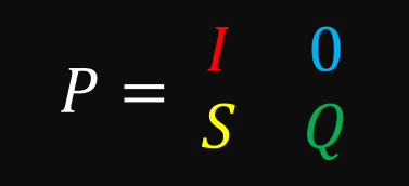
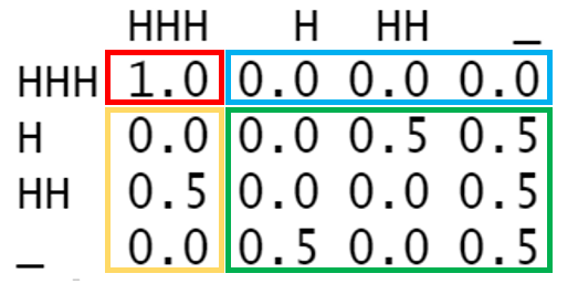
In the top left is an identity matrix with all of our absorbing states. Right now, this identity matrix only has a single item in it, but we’ll see later that even with multiple absorbing states, the top left quadrant always takes that form. In the top right, we see all 0’s. That should make sense because absorbing states, by definition, do not lead to other states. In the bottom left are all the transition probabilities leading to absorbing states from transient states. In the bottom right are all transition probabilities that lead from one transient state to another.

What happens when we square this matrix?

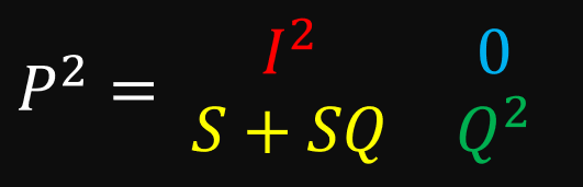
You can verify using matrix multiplication that the top 2 rows do not change. We can generalize this to any power:

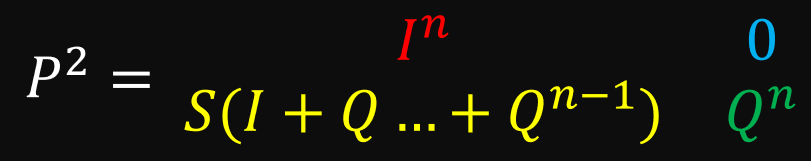
Notice that the bottom right quadrant gives us the same results as if it were its own matrix. Because this quadrant contains the transition probabilities we need (transient to transient), we can ignore the rest of the matrix.

This saves us some time, but our current solution still does not scale well for large matrices. We can do better. Try to take a minute to think about whether this process reminds you of anything you’ve encountered in the field of probability before.

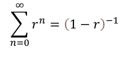
If what we just did reminds you of a geometric series, then you’re on to something, because that’s exactly it! Recall that the closed-form solution to a the sum of a geometric series is this:

Here is its cousin for matrices:

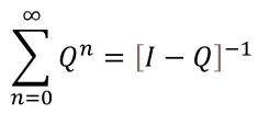
Of course, this equation only yields a solution when the sum converges, and, luckily, we know that happens. Let’s try it out in R:

Q <- coins[c("H", "HH", "_"), c("H", "HH", "_")]steps <- solve(diag(3) - Q)steps H HH _
H 4 2 6
HH 2 2 4
_ 4 2 8

Easy, right?

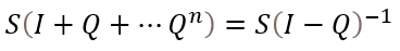
The last interesting portion of the matrix that we haven’t addressed is S. You might be able to be able to guess what S is based on the information we’ve gone over so far. If we raised the rearranged matrix to the 300th power to see its long term behavior, we get the following:

matrixpower(coins, 300)
HHH H HH _
HHH 1 0.000000e+00 0.000000e+00 0.000000e+00
H 1 3.438577e-12 1.869516e-12 6.324529e-12
HH 1 2.227506e-12 1.211071e-12 4.097023e-12
_ 1 4.097023e-12 2.227506e-12 7.535600e-12

So, it looks like S is just a bunch of ones… though this is not particularly exciting, it makes sense when you consider that S contains rows of transient start states in the column of the single absorbing state — which, as we have gone over before, should be the probability that a certain chain ends in a given absorbing state. Because we only have 1 absorbing state, this is the behavior we would expect (this implies we will eventually get three heads in a row).

Again, there’s no need to do some arbitrarily large number of matrix operations to get this distribution. We need only look as far as the equation we saw earlier.

Which gives us:

S <- coins[c(2, 3, 4), 1]steps %*% Ssteps [,1]
H 1
HH 1
_ 1

Game of Catch at the Beach 🌅

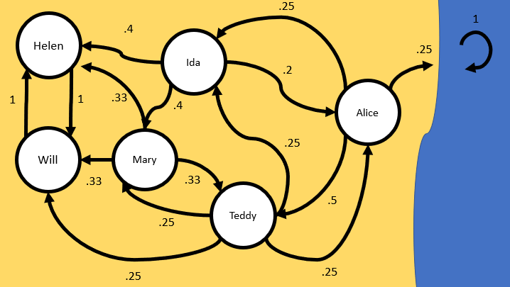
Now, let’s do a slightly more complicated example by playing a game of catch at the beach. Try to solve it yourself if you can (creating the matrix in R can be quite tedious, so you can skip ahead and use mine if you just want to plug in values to solve the problem):

Teddy passes a ball to Will, Mary, Ida, Or Alice with equal probability.

Mary passes to Teddy, Ida, or Will with Equal probability.

Ida passes to Helen or Mary with equal probability, and to Alice half as often as Mary.

Helen and Will only pass the ball to each other.

Alice passes to Teddy half the time, and then throws the ball to Ida or into the ocean (where it is never to be seen again) equally often.

1. What is the probability that the ball will end up with Will and Helen, given that Teddy starts with the ball?
2. How many times do we expect Alice to receive the ball if Ida starts with it?
3. On average, how many throws will the entire game last if Teddy starts with it (and we assume the game ends when the ball is lost or Helen and Will keep it forever)?

Drawing the state space as a graph is typically a good first step:

Then, we create a matrix in R. Rbind seems like the easiest for this scenario:

catch <- rbind(c(0, .25, .25, 0, .25, .25, 0), c(1/3, 0, 0, 1/3, 1/3, 0, 0), c(0, .4, 0, .4, 0, .2, 0),
c(0, 0, 0, 0, 1, 0, 0), c(0, 0, 0, 1, 0, 0, 0), c(.5, 0, .25, 0, 0, 0, .25), c(0, 0, 0, 0, 0, 0, 1))dimnames(catch) <- list(c("T","M","I","H", "W", "A", "O"), c("T","M","I","H", "W", "A", "O"))catch T M I H W A O
T 0.0000000 0.25 0.25 0.0000000 0.2500000 0.25 0.00
M 0.3333333 0.00 0.00 0.3333333 0.3333333 0.00 0.00
I 0.0000000 0.40 0.00 0.4000000 0.0000000 0.20 0.00
H 0.0000000 0.00 0.00 0.0000000 1.0000000 0.00 0.00
W 0.0000000 0.00 0.00 1.0000000 0.0000000 0.00 0.00
A 0.5000000 0.00 0.25 0.0000000 0.0000000 0.00 0.25
O 0.0000000 0.00 0.00 0.0000000 0.0000000 0.00 1.00

Now, the only real tricky thing is how to handle the recurrent class that has more than two states (Helen and Will). The solution is pretty elegant. We just treat them as a single state. Whether Mary throws to Helen or Will doesn’t matter, since the ball faces the same fate either way. The same goes for every other state transitions to Helen and Will. So, we just add columns H and W and then delete either row H or W (I’ll choose W this time).

WH_col <- catch[,"H"] + catch[,"W"]WH_col <- WH_col[-5]catch <- catch[c(-5), c(-5)]catch[,"H"] <- WH_colcatch["H",] <- catch["W",]catch T M I H A O
T 0.0000000 0.25 0.25 0.2500000 0.25 0.00
M 0.3333333 0.00 0.00 0.6666667 0.00 0.00
I 0.0000000 0.40 0.00 0.4000000 0.20 0.00
H 0.0000000 0.00 0.00 1.0000000 0.00 0.00
A 0.5000000 0.00 0.25 0.0000000 0.00 0.25
O 0.0000000 0.00 0.00 0.0000000 0.00 1.00

The rest is just like before:

catch_2 <- catch[c(6, 2, 3, 4, 5, 1), c(6, 2, 3, 4, 5, 1)]catch_2 <- catch_2[c(1,4, 3, 2, 5, 6), c(1, 4, 3, 2, 5, 6)]catch_2 O H I M A T
O 1.00 0.0000000 0.00 0.00 0.00 0.0000000
H 0.00 1.0000000 0.00 0.00 0.00 0.0000000
I 0.00 0.4000000 0.00 0.40 0.20 0.0000000
M 0.00 0.6666667 0.00 0.00 0.00 0.3333333
A 0.25 0.0000000 0.25 0.00 0.00 0.5000000
T 0.00 0.2500000 0.25 0.25 0.25 0.0000000Q <- catch_2[c("I", "M", "A", "T"), c("I", "M", "A", "T")]S <- catch_2[c("I", "M", "A", "T"), c("O", "H")]solve(diag(4) - Q) %*% SO H
I 0.07975460 0.9202454
M 0.03680982 0.9631902
A 0.32515337 0.6748466
T 0.11042945 0.8895706 # 89% chance the ball goes to Hsolve(diag(4) - Q)
I M A T
I 1.1656442 0.5521472 0.3190184 0.3435583 #A gets the ball .32 times
M 0.1533742 1.1779141 0.1472393 0.4662577
A 0.5214724 0.4049080 1.3006135 0.7852761
T 0.4601227 0.5337423 0.4417178 1.3987730sum((solve(diag(4) - Q))[c("T"),])2.834356 # note that if the game is defined to still continue when Helen and Will receive the ball, the expected time for the game to last is infinite

That’s it for this example, not much new conceptually.

Random Walk Through Outer Space 🛸

Assume a space ship navigates the undirected graph of planets below using a random walk (this implies all outgoing transition probabilities from a vertex are equal):

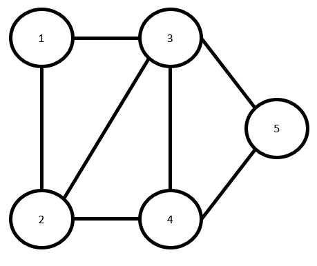
Assume the chain starts in state

1. What is the probability the ship reaches state 4 before it reaches state 5?

2. How many steps do we expect to take to get from state 2 to state 5 (in other words, what is the hitting time of state 5 from state 2)?

ship <- rbind(c(0, .5, .5, 0, 0), c(1/3, 0, 1/3, 1/3, 0), c(.25, .25, 0, .25, .25),
c(0, 1/3, 1/3, 0, 1/3), c(0, .5, 0, .5, 0))
ship
[,1] [,2] [,3] [,4] [,5]
[1,] 0.0000000 0.5000000 0.5000000 0.0000000 0.0000000
[2,] 0.3333333 0.0000000 0.3333333 0.3333333 0.0000000
[3,] 0.2500000 0.2500000 0.0000000 0.2500000 0.2500000
[4,] 0.0000000 0.3333333 0.3333333 0.0000000 0.3333333
[5,] 0.0000000 0.5000000 0.0000000 0.5000000 0.0000000

Again, there’s a simple trick to solve this problem. To find out the probability of reaching one state before any other, we need only turn both states into absorbing states and use known methods from there.

ship[c(4,5),] <- rbind(c(0,0,0,1,0), c(0,0,0,0,1))ship <- ship[c(5, 4, 3, 2, 1), c(5, 4, 3, 2, 1)]ship [,1] [,2] [,3] [,4] [,5]
[1,] 1.00 0.0000000 0.0000000 0.00 0.0000000
[2,] 0.00 1.0000000 0.0000000 0.00 0.0000000
[3,] 0.25 0.2500000 0.0000000 0.25 0.2500000
[4,] 0.00 0.3333333 0.3333333 0.00 0.3333333
[5,] 0.00 0.0000000 0.5000000 0.50 0.0000000Q <- ship[c(3, 4, 5), c(3, 4, 5)]
S <- ship[c(3, 4, 5), c(1, 2)]solve(diag(3) - Q) %*% S
[,5] [,4]
[1,] 0.3846154 0.6153846 # 62 percent chance to end in state 4
[2,] 0.2307692 0.7692308
[3,] 0.3076923 0.6923077

Problem 2 is nearly the same as before. We just need to turn a single state into an absorbing state:

ship <- rbind(c(0, .5, .5, 0, 0), c(1/3, 0, 1/3, 1/3, 0), c(.25, .25, 0, .25, .25),
c(0, 1/3, 1/3, 0, 1/3), c(0, .5, 0, .5, 0))ship[5,] <- c(0,0,0,0,1)ship <- ship[c(5, 2, 3, 4, 1), c(5, 2, 3, 4, 1)]ship [,1] [,2] [,3] [,4] [,5]
[1,] 1.0000000 0.0000000 0.0000000 0.0000000 0.0000000
[2,] 0.0000000 0.0000000 0.3333333 0.3333333 0.3333333
[3,] 0.2500000 0.2500000 0.0000000 0.2500000 0.2500000
[4,] 0.3333333 0.3333333 0.3333333 0.0000000 0.0000000
[5,] 0.0000000 0.5000000 0.5000000 0.0000000 0.0000000Q <- ship[c(2, 3, 4, 5), c(2, 3, 4, 5)]S <- ship[c(2, 3, 4, 5), 1]steps <- solve(diag(4) - Q)sum(steps[2,])6.333333

That’s it for this tutorial! Thank you so much for reading. Please send me any questions you have.

Further Reading

Introduction to Stochastic Processes with R by Robert P. Dobrow

Introduction to Stochastic Processes by Gregory F. Lawler