With nothing but a good model, a few definitions, and some math, we’ll derive a fundamental relationship of chemistry.

Anyone who has ever taken a chemistry class has seen the Ideal Gas Law:

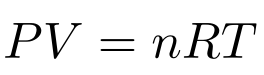
Chemistry classes tend to teach the Ideal Gas Law as a combination of Boyle, Charles, Gay-Lussac, and Avogadro’s Laws. Although they derived these laws empirically, we’re going to take a different approach in this article. We’re going to derive the Ideal Gas Law from nothing but statistical mechanics, a few laws, and some definitions. We’re going to use the concept of entropy, so check out my article on entropy if you’re unfamiliar with entropy. If you think entropy measures disorder, check out the article because it doesn’t.

The Rules

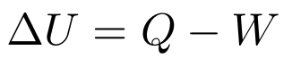
For this derivation, I will only use the definition of an ideal gas, the Laws of Thermodynamics:

• First Law: In a closed system, the change in internal energy is equal to the heat put into the system minus the work the system does on its environment.

• Second Law: An isolated system will tend towards its most likely macrostate.

(I won’t need the Third Law and I won’t use the Zeroth Law directly, so I’ve left them out.)

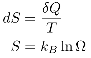
both definitions of entropy:

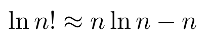
the Fundamental Counting Theorem (I’ll explain in a later section), Stirling’s Approximation:

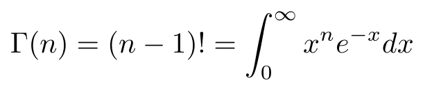
the Gamma Function:

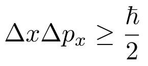
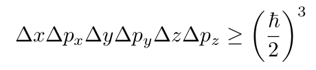
the definitions of work, pressure, temperature, volume, and number of particles, and (sort of) the Heisenberg Uncertainty Principle:

I’ll go into more detail about why we sort of need the Heisenberg Uncertainty Principle when it comes up.

What is an Ideal Gas?

An ideal gas is a gas of uniform particles whose particles do not interact and do not take up space. Although no gas has these properties, many gases consist of particles that rarely interact and take up a negligible amount of space. Ideal gases can approximate these gases over a wide range of values of pressure, volume, temperatures, etc.

If you want a video demonstration, here you go:

The Multiplicity of an Ideal Gas

Since we want to calculate entropy with statistical mechanics, we need to calculate the multiplicity of an ideal gas. The multiplicity represents the number of ways you can change the system under some constraints. In the case of the ideal gas, we’re looking at the number of ways you can choose the positions and momenta of the particles given a pressure, a temperature, the number of particles, and a volume.

We will look at one particle first to get a foothold in what we have to consider with the multiplicity. Then, we will move onto a many particle system.

One Particle

Let’s consider some thermodynamic variables and how we can use them to help us.

• Number of Particles: We’ve already used this when we established that we were using one particle.
• Volume: Since particles in our model can only move inside the given volume, the volume constrains the total number of possible positions.
• Temperature: Temperature is a measure of the average kinetic energy of a gas. Since it’s trivial to convert to internal energy through entropy or the Equipartition Theorem, we won’t need it.
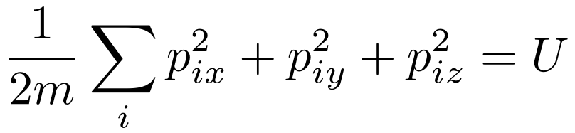
• Internal Energy: The sum of all the kinetic energies of the particles must equal the internal energy. We can use kinetic energy to find momenta, so the internal energy constrains the total number of possible momenta.
• Pressure: I don’t see how we can use pressure to get us something without us putting in significant effort. We’ll skip it for now.

Finding the Number of Possible Positions

We won’t be able to get an exact number of all possible positions since space is continuous (as far as we know). We can say that if we have twice the volume, we have twice the number of positions as we did before, so we can say

Finding the Number of Possible Momenta

As with position, we won’t be able to get an exact number of all possible momenta. The derivation is going to be a little weirder. As we said before, the sum of all the kinetic energies of each particle must equal the internal energy, which leaves us with

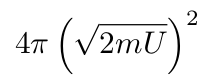
As weird as this looks, this equation describes the surface of a sphere. The number of possible momenta is proportional to the surface area of a sphere with a radius of the square root of 2mU.

Why Does a Sphere Show up in the Derivation?

If we look at the equation for kinetic energy, it only contains the magnitude of the momentum, so any momentum with that magnitude is possible. The set of all possible vectors with a given magnitude is the formal definition of a sphere, so that’s where we get the sphere.

The Equipartition Theorem

The system has no reason to give one component of kinetic energy more energy than any other component. Therefore, we assume that the energy of the system is spread evenly among all components of kinetic energy. This assumption is the Equipartition Theorem. While this theorem doesn’t hold when quantum effects are significant, it holds in classical mechanics. I’m mentioning the Equipartition Theorem so that we can assume that the system can be any point on the sphere with the same probability.

The Fundamental Counting Theorem

The Fundamental Counting Theorem states

If there are m outcomes for one event and n outcomes for an independent event, there are mn possible outcomes for the combined event.

For example, if you roll a die, you have six possible outcomes ({1, 2, 3, 4, 5, 6}). If you flip a coin, you have two possible outcomes ({H, T}). If you roll a die and flip a coin, you have twelve possible outcomes ({H1, H2, H3, H4, H5, H6, T1, T2, T3, T4, T5, T6}).

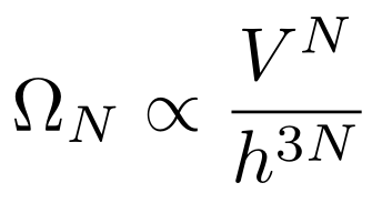
In our case, we have m possible positions and n possible momenta, so we have mnpossible microstates. Since m is proportional to the volume and n is proportional to the surface area of the sphere, the multiplicity is proportional to

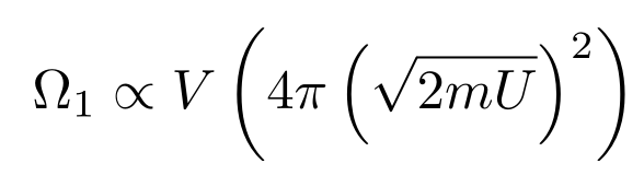
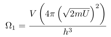
Removing the Units

If I asked you how many possible outcomes you could have for something happening, you could say two or two million, but you couldn’t say two million meters. The number of anything can’t have units behind it, which presents us with a problem since our multiplicity has units of Joule³ Seconds³. To get rid of this, we can divide by some constant with units of Joule³ Seconds³. h³ has the right units and kind of makes sense since the Heisenberg Uncertainty Principle states

If we include all three dimensions, we end up with

which is volume times momentum cubed, so you can imagine chopping up the momentum-position space into “cubes” with a size of h³.

Why h instead of h/4π?

I’ve never seen an adequate explanation for why Sackur and Tetrode chose to use h³ instead of (h/4π)³. Before Heisenberg’s Uncertainty Principle, everyone tended to solve problems by restricting things to integer multiples of h or h/2π (e.g. Planck’s Blackbody Equation, the Bohr atom, etc.). I think Sackur and Tetrode did the same without a theoretical reason. I found someone on the internet saying that you can also get some mathematical justification for hinstead of h/4π by expanding out some quantum density matrix, but I wasn’t able to see it in the source the person named. Furthermore, he was the only source I could find online that gave a reason besides (it has the right units). If anyone has a strong reason for using h instead of h/4π, let me know in a response to this article.

Back to the Multiplicity

Regardless of what we choose, the exact value of the entropy won’t matter for our purposes, as we’ll focus only on differences in entropy. At this point, we now have the following expression for the multiplicity of a singular particle:

Problem with the Units

This expression doesn’t have the right units. 2mU is momentum² and we need momentum³. We can fix this issue by either multiplying by a constant or raising the square root of 2mU to the power of three. Once we start working with a large number of particles, we’ll choose the second option. I’ll explain more when we get to that section. For now, I’m going to leave it and move on.

Multiple Particles

We can use the Fundamental Counting Theorem for any independent quantities.

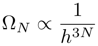
Constants

Since constants are independent of the system, we will divide the multiplicity by h³ for each of the N particles, leaving us with

Positions

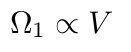
As I said earlier in my definition of an ideal gas, the particles do not take up space and do not interact. The position of each particle is therefore independent of any other particle. Since we have independent positions, we will multiply the multiplicity by V for each particle, leaving us with

Momenta

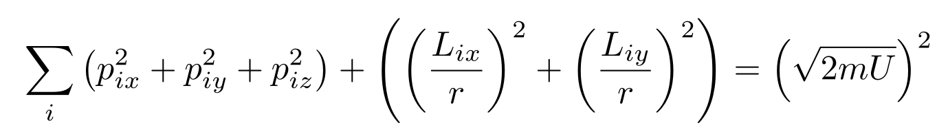
Unlike the constants and the positions, the momenta depend on each other. Consider the kinetic energies of each particle with respect to the total energy.

Remember that we’re looking for the number of possible ways to distribute momenta for a given amount of energy. If we change the energy to X Joules, then we’re looking for the number of possible ways to distribute momenta such that the total amount of energy is X Joules. For this reason, we consider the energy to be constant in this part of our analysis.

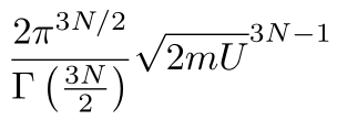
The next part sounds worse than it actually is. If we look at the momenta terms, we have a bunch of squared values adding up to a constant. If we had two squared values adding together to get a constant, we would have a circle. If we had three squared values, we would have a sphere. We have more than three squared values, though, so we have a hypersphere. To find the multiplicity of the momenta, we need to find the surface area of an n-dimensional hypersphere. Don’t freak out, though. Math allows us to talk about things without seeing them. If we trust the math, we can make our way through this problem. Before we go any further, I recommend checking out 3Blue1Brown’s video Thinking outside the 10-dimensional box. In our case, we are looking for the surface area of a sphere with 3N dimensions and radius of the square root of 2mU.

Hyperspheres

There are many ways to find the surface area of an n-dimensional sphere. I’d rather not do the direct integral in this derivation since I’d have to cover hyperspherical coordinates. Instead, we’ll use properties of n-dimensional spheres. We’ll need three facts:

• We can express an n-dimensional sphere as a sum of squares adding up to a radius squared.
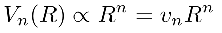
• The volume of any n-dimensional object is proportional to its radius raised to the nth power.

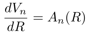
• The surface area is the derivative of the volume in any dimension with respect to the radius. (For squares and cubes, the “radius” is any length from the center to a point on the surface of the cube.)

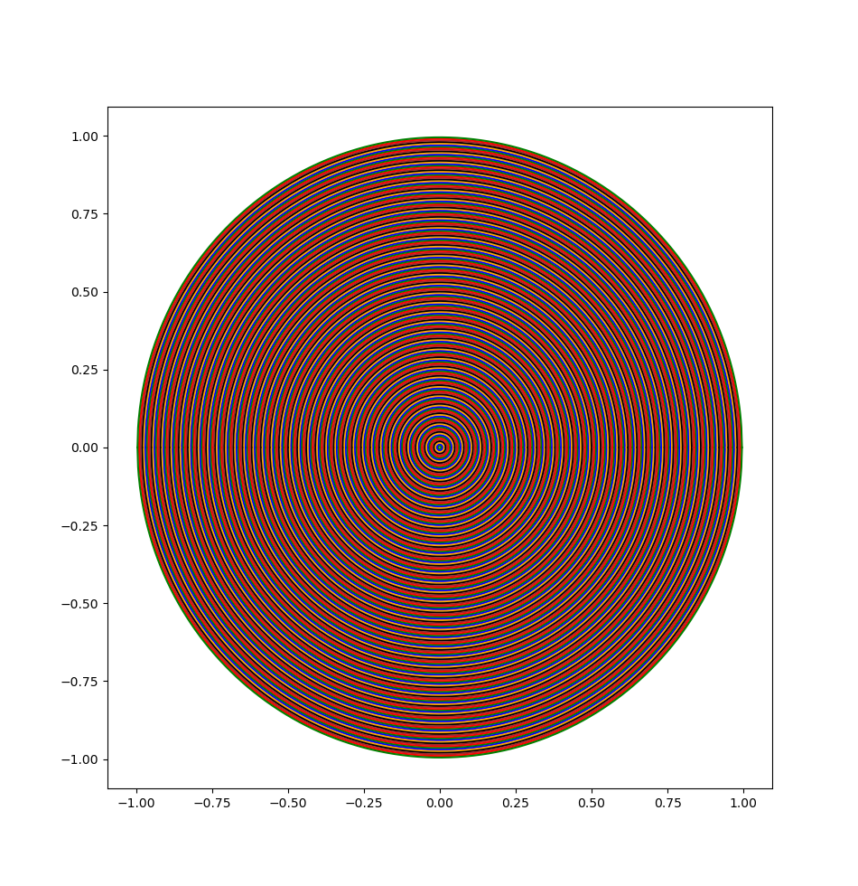
The proportionality relationship should make sense. You need units of length to the n for n-dimensional volume and volume should increase as the radius increases. The relationship between surface area and volume should also make sense. Imagine painting a ball bearing with thousands of layers of paint. Each layer increases the volume of the ball by a small amount while still keeping it spherical. If you kept adding layers, you would get a sphere as large as the Earth. If you want a visual example in 2D, take the following image:

If we combine the last two facts, we end up with

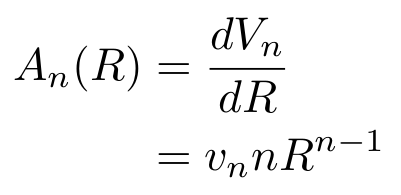
With this result, we can see that we only need to find vn to get our answer.

Our Plan for the Hypersphere

1. We’re going to come up with two different expressions that equal each other. One of these ways will contain vn and the other will not. Both the sum of squares and the n-dimensional volume differential element (dVn) need to show up in at least one of these expressions.
2. We can then set these two expressions equal to each other and solve for vn.

Sum of Squares in One of the Expressions

We’ll want to be able to add as many squares as we would like, so we’ll look for a function f and an operation ★ (addition, subtraction, multiplication, division, or any function that takes in two values and spits out another value) that satisfies f(a + b) = f(a) ★ f(b). If we find such a function and operation, then

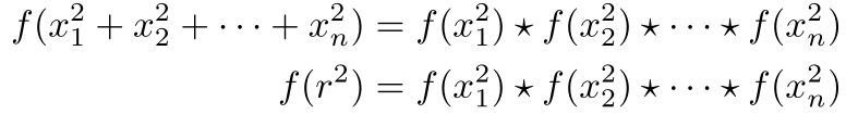
This equation will allow us to work with f(r²) and f(x²), which can make our job easier.

If we let ★ be addition and f(x) = x, then we’ll end up integrating in hyperspherical coordinates, which I wanted to avoid. I can’t see any other way to satisfy the above restrictions on f with ★ being addition than to let f(x) = x, so let’s try something else. Subtraction won’t work since f(a + b) = f(b + a), which means f(a) ★ f(b) = f(b) ★ f(a). In math terms, ★ must be commutative. Since subtraction isn’t commutative, we can’t use it. Same goes for division. Multiplication is the only basic operation we have left. In that case, we want some function that satisfies f(a + b) = f(a) f(b).

I don’t want to beat around the bush too much, so we’ll take f(x) to be an exponential function. I don’t care if f(x) could be anything else since exponential functions will work. Since we’re working with calculus, we’ll want to work with e (Euler’s number) or 1/e being the base. These two numbers have nice properties. We have two main contenders: f(x) = exp(x) (e is the base) and f(x) = exp(-x) (1/e is the base). Since x² is always positive, exp(x²) will go to infinity as x goes to infinity, which makes the integral harder to evaluate. On the other hand, exp(-x) goes to zero as x goes to infinity, so we’ll take f(x) = exp(-x).

Volume Differential Element in One of the Expressions

So now, we just need an expression with dVn. The dVn suggests an integral or a derivative. We’re dealing with volumes, so we’ll try the integral. Remember that we’re working with exp(-x²), which has the famous integral

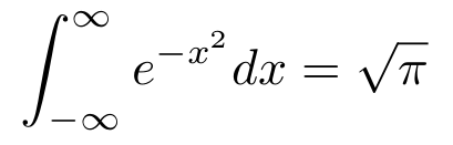
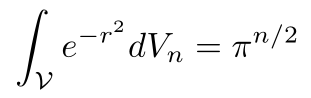
I’ll link to a proof since I wouldn’t be able to add anything. If you want to derive it on your own, look for a similar integral that you can integrate (say if you multiplied the integrand by x) and try to convert the original integral into the easier integral. You might want to look into polar coordinates since dA = r dθ dr and you could use that r or look into the Leibniz Rule/Feynman’s Differentiation Under the Integral. Anyway, if we multiply n Gaussian Integrals, we can use f(a) f(b) = f(a + b) and we end up with

We’re integrating over the x’s, so we can call them whatever we like without changing the value of the integral. Regardless, we have a sum of squares in the left half and our right half is a known value.

To use this equation, we’ll need to make a few notes and come up with some definitions. First, note that the integral is over all space in n dimensions. We’ll use something to denote the region independent of the coordinate expression. Second, note that the combination of all the dx’s is a volume element in n dimensions, i.e. dVn. Lastly, we can use the fact that the sum of squares equals r². As a quick summary:

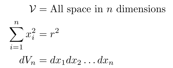
Putting it all together gives us

Solving for vn

Now, we’ll use the relationship between dVn and dr:

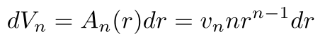
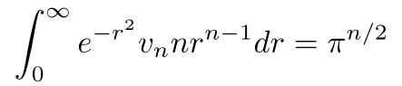
Substituting it back into the integral and setting the appropriate bounds (r = 0 to r = ∞) leaves us with

Now, we do a little bit of algebra and calculus

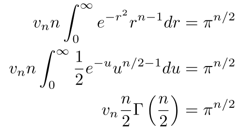
We let u = r² for a u-substitution, then we recognized the definition of the gamma function, the analytic continuation of n!. You can think of the gamma function as connecting all the values of n! with a smooth curve. In specific terms, Γ(n) = (n - 1)!. If you’d like a proof, you could use a proof by induction with integration by parts.

Note that Stirling’s Approximation applies to the Gamma Function as well as it does to the factorial. We’ll make use of this fact later. At this point, if we solve for vn, we can get the volume and the surface area.

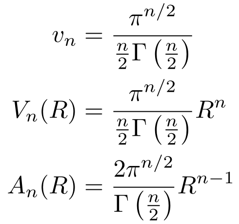
Plug in n = 2 and you get the circumference and area of a circle. Then plug in n = 3and you get the surface area and volume of a sphere.

Plugging in our specific values for the radius and the number of dimensions, we get

Double Counting

Say that we have two particles for now. Each has a specific momentum and position. Say we switch the two particles so that the first particle has the position and momentum of the second and vice versa. Both these situations describe the same microstate, meaning we have to divide by 2. If we didn’t divide by 2, we would count this state multiple times. With more particles, any permutation will describe the same microstate. We have to divide our multiplicity by the number of permutations, N! to avoid counting the same microstate multiple times. If we don’t account for the indistinguishable particles, we could violate the Second Law of Thermodynamics.

The Multiplicity of a Monatomic Ideal Gas

Putting everything together, we have:

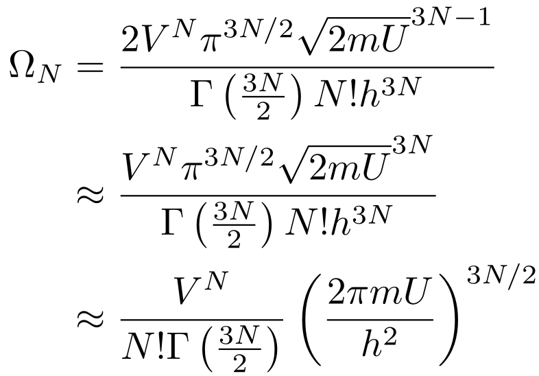
I made two simplifications. First, the 2 out front adds a small constant to the entropy that we can ignore. Second, I have increased the power of the square root of 2mU by 1 since we’re dealing with very large numbers and we need the units to work out. You can imagine this as converting a surface area to a volume by multiplying by a small thickness. If you want to see why these approximations work, don’t make them and see the difference between the values (remember that N is on the order of 10²³). Other than that, I cleaned up the expression.

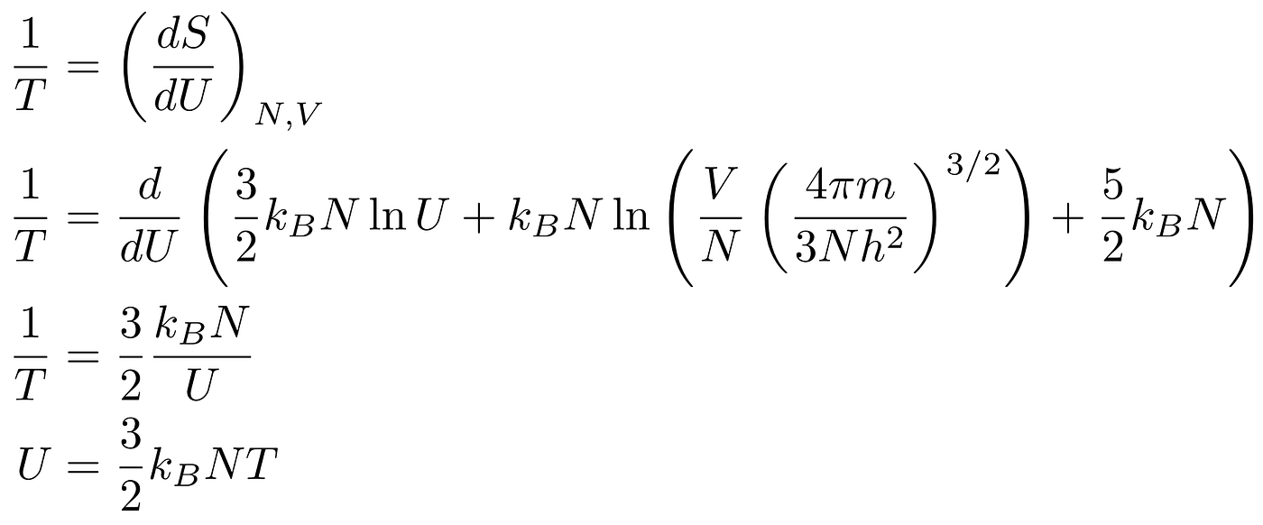
The Entropy of a Monatomic Ideal Gas

Now that we have the multiplicity of an Ideal Gas, we can use it to find the entropy:

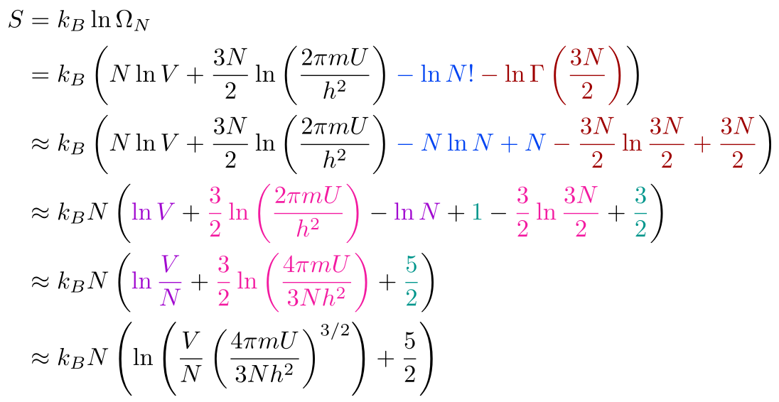
We went from the first line to the second line by substituting in the multiplicity for N particles. Then, we used logarithm rules to split up products. Then, we applied Stirling’s approximation so we ended up with N ln N - N instead of ln N!. Since Γ(n) = (n - 1)!, we can also use Stirling’s approximation. We can ignore the -1 in Stirling’s approximation of the gamma function since n >> 1 (Don’t approximate if you don’t believe me and check the accuracy of the approximation.). Then, we factored out N, added 3/2 and 1 to get the 5/2, brought the two terms with a 3/2 in front into one logarithm, and combined the two remaining logarithms. For the last line, we combined all the logarithms into one logarithm. We have derived the the Sackur-Tetrode Equation for the entropy of an Ideal Gas! We’re quite close to the Ideal Gas Law, but we’ll need to do some more work (pun not intended and not funny) to get pressure and temperature into our math.

The First Law of Thermodynamics

Now that we have the Sackur-Tetrode Equation, we can use the First Law of Thermodynamics to derive the Ideal Gas Law. In its current form, the First Law of Thermodynamics can’t help us much, so we’ll have to rewrite it in terms of temperature, entropy, pressure, and volume. First, we’ll rewrite both sides in terms of differentials

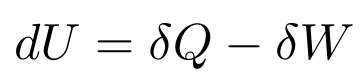
where dU is an exact differential and both 𝛿Q and 𝛿W are inexact differentials.

Exact and Inexact Differentials

The integral of an exact differential only depends on its endpoints (a.k.a. path independence) while an inexact differential depends on how you get from one endpoint to another. As a practical example, gravitational potential energy is an exact differential. If you lift a weight in the air, you’ve increased its potential energy. If you put it back down, you’ve decreased its potential energy back to its original value. You, on the other hand, have lost energy lifting the weight and putting it back down. The work must therefore be an inexact differential. As this Khan Academy article explains (at the end), your body is doing work to keep the tension in your muscles. To calculate the work done, you would have to do the work integral and account for efficiency.

We’ll end up with exact differentials in the next step, so the distinction doesn’t matter for us.

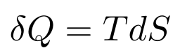
Heat in Terms of Entropy and Temperature

Given the definition of entropy, this part is trivial:

Work in Terms of Pressure and Volume

Work depends on force and distance, so we’re going to need some way of getting force and distance from pressure and volume. We can get a pretty good guess by looking at the units. Pressure is [force] / [distance]² and volume is [distance]³. We want [force] ꞏ [distance]. If we multiplied pressure and volume, we would get something with the right units. How do we know that their product is work?

Consider a piston.

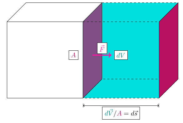
The piston pushes an object with a force over a distance through expansion (a.k.a. a change in volume). If we think about the side of the piston that pushes the object, we’ll have an area. With force and area, we get pressure. With area and distance, we get volume.

The little s is the path element and it’s an infinitesimal distance with a direction. Pressure always points in or out of the surface, so it’s always in the same or opposite direction as the volume change. Regardless, we can turn the dot product into a regular product of their magnitudes. We end up with

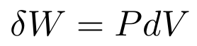
This principle applies to far more than just pistons. If you imagine a small square on a balloon, you can treat it like the piston above.

What About Changes in Pressure?

If the volume doesn’t change, then the force is applied over zero distance, so no work is done. If the pressure changes as the volume changes, then we can rewrite pressure as a function of volume. If the volume is constant but the pressure changes, any change in the internal energy will show up as heat.

Putting it all Together

At this point, we have

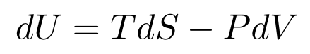
This equation is the Fundamental Thermodynamic Relation.

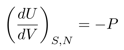
Some Useful Derivatives

For the moment, let’s say that we keep the system at constant volume. In that case, we recover the definition of entropy:

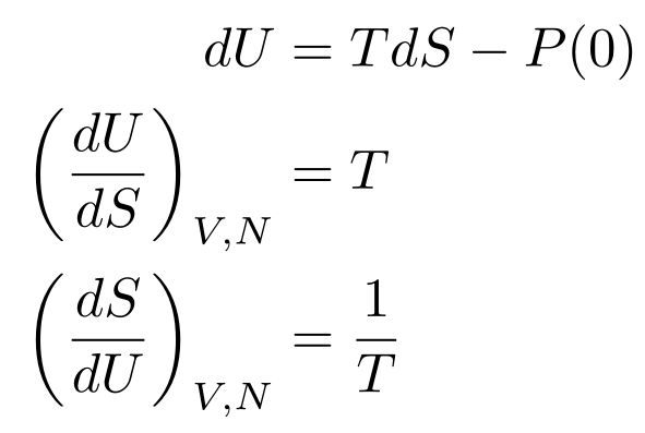
The subscript outside the parentheses means we kept that variable constant. In this case, we kept the volume and the number of particles constant. Since you usually get entropy as a function of total energy, the second derivative is used more often.

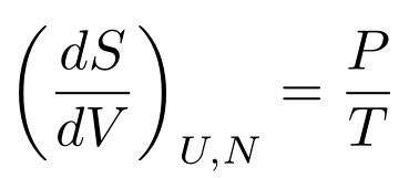
Now, let’s say that we keep the entropy constant. We then have a useful relationship between pressure, volume, and internal energy:

Let’s say the internal energy is constant. We then have a useful relationship between entropy, temperature, pressure, and volume:

We can only use these derivatives if we can assume something is constant, however. Luckily for us, we can use the Second Law of Thermodynamics.

Sidenote: Technically not Dividing the Differentials

If you’re a mathematician, then we’re either doing nonstandard analysis or using the chain rule/u-substitution (same thing) to get the derivative out of the result.

I’m taking a shortcut because we’re doing physics, not rigorous real analysis.

The Second Law of Thermodynamics

If you change any of the macroscopic properties fast enough, the rest will take some time to catch up. If you expanded the piston from earlier at half the speed of light, part of the added volume would be empty. At that point, it doesn’t make sense to talk about the pressure or temperature of the entire system since it varies throughout the system. In a similar manner, if we added particles or energy in one corner of a box, we would also have differences in pressure throughout the box and it no longer makes sense to talk about the pressure or temperature of the system. In any of these cases, we couldn’t use any law that relies on one uniform pressure or temperature throughout the system. We have to restrict ourselves to the specific case of thermal equilibrium.

The Second Law of Thermodynamics guarantees that there is a thermal equilibrium for an isolated system: the most likely macrostate. If we’re in thermal equilibrium, none of the macroscopic properties (pressure, volume, number of particles, temperature, internal energy, and entropy) of the system will change.

You might worry that we can’t use the derivatives since all the variables are constant, but that means dS, dV, dU, etc. are all “zero” (technically limits approaching zero), which they were anyway by virtue of being differentials.

We could probably try to maximize the entropy, but I don’t think we’d get too much out of it.

Deriving the Ideal Gas Law

We can assume constant energy, which means we can use one of the derivatives we derived in the section on the First Law of Thermodynamics:

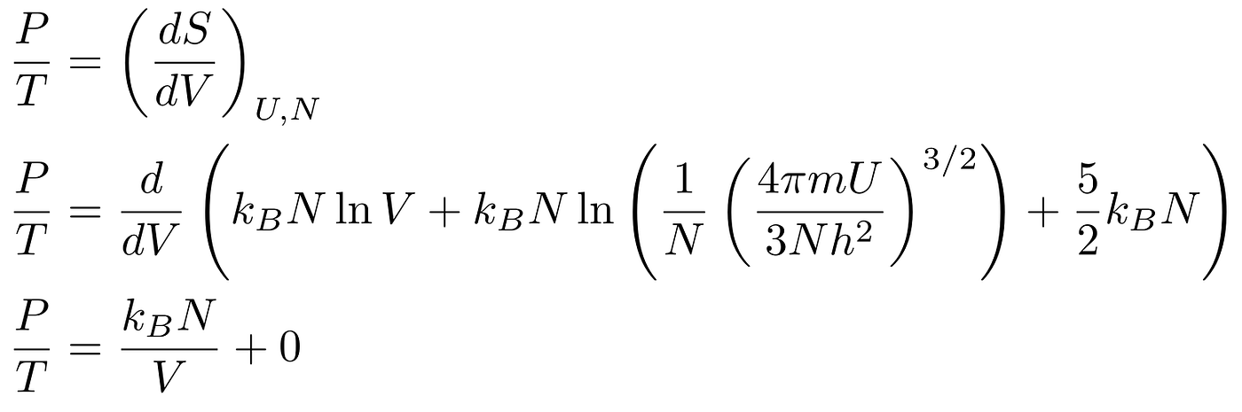
Some algebra yields the Physicist’s Ideal Gas Law:

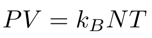
If we make the substitutions R = kB A (where R is the Ideal Gas Constant and A is Avogadro’s number) and n = N/A, we end up with the Chemist’s Ideal Gas Law:

Q.E.D.

Internal Energy of an Ideal Gas

We can also get some useful quantities, such as an exact expression for the internal energy of the gas. If we assume constant volume, we get:

What About Gases with More Atoms per Particle?

With multi-atomic gases, you still have volume and momenta, but now you have to consider angular momenta, orientation, and energy from vibrations. Because the position is independent of everything else, the multiplicity will still be proportional to V to the N. The Ideal Gas Law still holds.

There are more ways to distribute energy (a.k.a. degrees of freedom) for multi-atomic gases, so the expression for the internal energy changes. Since rotational kinetic energy and bond energy (modeled as a spring) are both represented as some constant times a number squared, we end up with something like the following for diatomic molecules:

I neglected one of the angular momenta components because the moment of inertia for the bond axis is so high that the molecule will not rotate around it for most reasonable temperatures. Quantum Mechanics restricts systems to discrete states, so the bond axis component of angular momentum must either be zero or a large number for the system. In a similar manner, low temperatures will end up freezing the energy stored in the bond at a fixed number, so you’ll end up with

In the first case where bond energy can vary, we have a 6N dimensional sphere. In the second case where bond energy is fixed, we have a 5N dimensional sphere. In either case, we need the surface area of the hypersphere. Since no other term contains the internal energy, you end up with

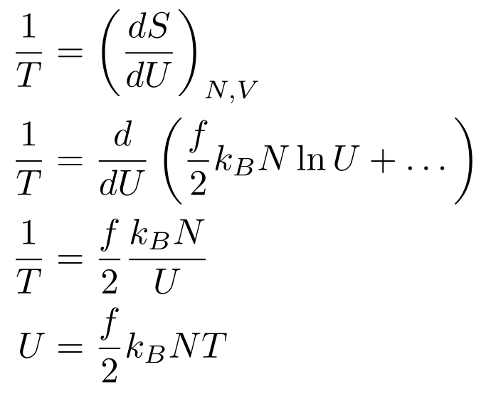
where f is the degrees of freedom (6 with bond energy and 5 without the bond energy).

We also need the orientation and how far the bond is stretched in the multiplicity, so we have a few more terms. We also add some more h’s in the denominator because each position-momentum component pair has an uncertainty principle. Regardless, the Ideal Gas Law and the Equipartition Theorem still hold, so it doesn’t matter for this derivation. For multi-atomic gases, you would be better off measuring quantities than calculating them.

Addendum: Chemical Reactions

If we had any chemical reactions happening (say in a car’s engine), we would also add some chemical potential terms for each chemical in the system to the Fundamental Thermodynamics Relation like so:

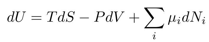
Each μ represents the chemical potential energy for each chemical in the system. Each dN represents the change in the amount of each chemical in the system.

Ideal gases do not have chemical reactions, so we left the chemical potential terms off.

Why Go through all this Trouble?

Benoît Paul Émile Clapeyron had derived the Ideal Gas Law decades earlier using the empirical observations of Boyle, Charles, Gay-Lussac, and Avogadro. So why go through this proof? Why not use Clapeyron’s proof and move on?

Understanding

Nothing promotes understanding like practical application. As I said in my power rule article:

Students tend to see math as a list of random facts to memorize with little to no connection between them.

This mindset applies to almost all fields of study, including physics. Students should feel as if each topic flows into every other topic — that they can learn new things from what they already know. By giving this proof, we can see the relationship between all these thermodynamic quantities. We see how to use the tools of statistical mechanics and thermodynamics to get useful results.

Consistency

If we had done this derivation and ended up with anything but the Ideal Gas Law, we would have to rebuild a large section of thermodynamics. One of the laws or theorems used in the derivation must have been wrong, and we would have to modify the erroneous law or theorem. In a way, this proof was an experiment to verify all the theorems and laws we used in this proof.

Ideal Gas Constant

Let’s say you derive the Ideal Gas Law purely through empirical means. Why does the Ideal Gas Constant (R) have a value of around 8.314 J / (K · mol)? We’re not done yet, though. If we look at the Dulong-Petit Law, we get that the molar heat capacity (the amount of energy required to raise the temperature of 1 mole of atoms by one Kelvin) of most solids is usually around 24.942 J / (K · mol), or 3 R. Why does the Ideal Gas Constant show up in the molar heat capacity for solids?

Without statistical mechanics (either by using the Equipartition Theorem or going through this same process of deriving the entropy of an Einstein or Debye solid and taking the high-temperature approximation), you can’t explain why these two values are related. It’s a happy coincidence and nothing more.

Practical Applications of Math

I can’t stand the question “When am I ever going to use this?” for many reasons, but I’ll focus on one here: I don’t know when anyone is going to use anything in math or science. If I did know every possible use for each mathematical concept, I would stop global warming, cure every single disease, end poverty and hunger, unify the four fundamental forces, solve the six remaining Millennial problems, build an interdimensional warp drive, etc.

What we consider impractical with our limited foresight may turn out to be not just practical, but fundamental to our understanding. I could list thousands of examples, including number theory leading to modern cryptography, curved manifolds leading to Einstein’s General Relativity, gambling games leading to probability leading to Quantum Mechanics, etc., but I won’t. Instead, I’ll use this article as an example.

Before this article, could you name a practical application of knowing the surface area of an n-dimensional sphere? In a similar manner, do you think the mathematician who derived the formula knew that you could use it to derive the Ideal Gas Law? Even if you knew statistical mechanics, would you have thought you would need the surface area of an n-dimensional sphere? I’d bet money on “no” to all these answers. After reading this article, do you think the formula for the surface area of an n-dimensional sphere is useless?

To be clear, I’m not saying everyone is going to use the formula in their daily lives. In fact, I doubt most people will ever use it. I’m saying that you don’t know what’s going to be useful before you need to use it.

Conclusion

If you’d like to see more discussions about entropy, check out my other two articles on the subject: Stop Saying Entropy is Disorder and Creationism and Entropy. If you want to see another derivation from scratch, check out my article Let’s Derive the Power Rule from Scratch. If you want an entire series with a similar style and mathematical rigor, check out The Road to Quantum Mechanics. If you’d like to see me derive something else from scratch, leave a suggestion in a response to this article and I’ll see what I can do.