Huber Loss: Why Is It, Like How It Is?

On the day I was introduced to Huber loss by Michal Fabinger, the very first thing that came to my mind was the question: “How did someone joined these two functions in a mathematical way?”. Apart from that, the usage of Huber loss was pretty straightforward to understand when he explained. However, he left me with enough curiosity to explore a bit more about its derivation. This poor excuse for an article is a note on how I explained my self the answers I obtained for my questions. I sincerely hope this article might assist you in understanding the derivation of Huber loss a bit more intuitively.

Huber loss function is a combination of the mean squared error function and the absolute value function. The intention behind this is to make the best of both worlds. Nevertheless, why is it exactly like this? (For the moment just forget about getting the mean).

If we are combining the MSE and absolute value function, why do we need all those other terms, like the -δ² and the co-efficient 2δ . Can’t we keep the function as follows ?

Well, the short answer is, No. Why? Because we need to combine those two functions in a way that they are differentiable. It’s also necessary to keep their derivatives continuous obviously because its use cases are associated with derivations (E.g.- Gradient Descent). So let’s dig in a little bit more and find out why does it have to be in this form?

Our intention is to keep the junctions of the functions differentiable right? So let’s take a look at the joint as shown in the following figure.

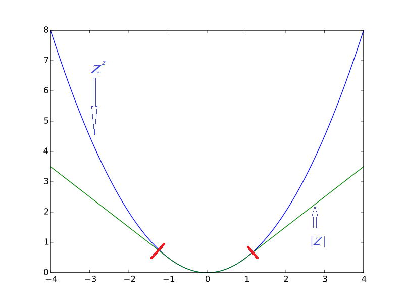
The joint can be figured out by equating the derivatives of the two functions. Our focus is to keep the joints as smooth as possible. This becomes the easiest when the two slopes are equal. So let’s differentiate both functions and equalize them.

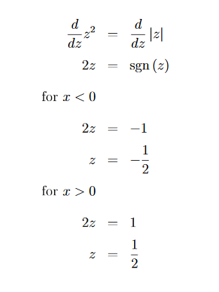
(More information about the signum / sign function can be found at the end)

This is useful to understand the concept. But, in order to make some use of it, we need to have a parameter in the function to control the point where we need to switch from one function to the other. In other words, we need to have a handle on the junction of the two functions. That’s why we need to introduce δ . For the convenience of this calculations, let’s keep the z² function unchanged and change the second case. Therefore δ should be introduced to the second function(associating the absolute value function). I guess the other way around is also possible. But there could be reasons why it’s not preferred. Your feedback on this is appreciated.

So hereafter I would be referring to the second case of the Huber loss as the second function since that’s what we are trying to generate here.

For easier comprehension, let’s consider for the case of z>0 only at this time. Let’s say we need to join the two functions at an arbitrary point δ. Two main conditions which need to be satisfied here are as follows.

At z= δ ,

1. the slope of z² should be equal to the slope of the second function.
2. value of z² should be equal to the value of the second function.

Based on condition (1), let’s find out the slope of function z² at z= δ .

Now we need to find a linear function with this gradient( 2 δ ) so that we could extend z² from z= δ to ∞ . The function with this gradient can be found by integration.

Here c is an arbitrary constant. So in order to find c let’s use condition (2).

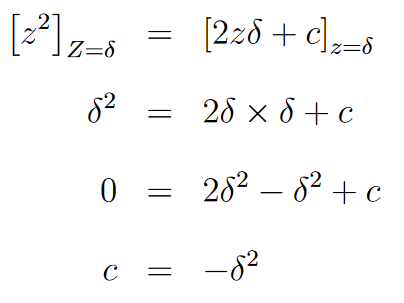
So there we have it ! The second function can be conclusively written as 2δz- δ²for the case of z>0 . We can do the same calculation when z<0 as well. Since the functions are symmetrical along z=0 , we can use the absolute value function for the second case. Then the final Huber loss function can be written as follows.

In Wikipedia you can see the same formula written in a different format:

Here you can think about it as they have started the process by keeping (1/2)z²unchanged, opposed to z² which I used in this derivation. As an exercise you can try to derive the second function by starting from,

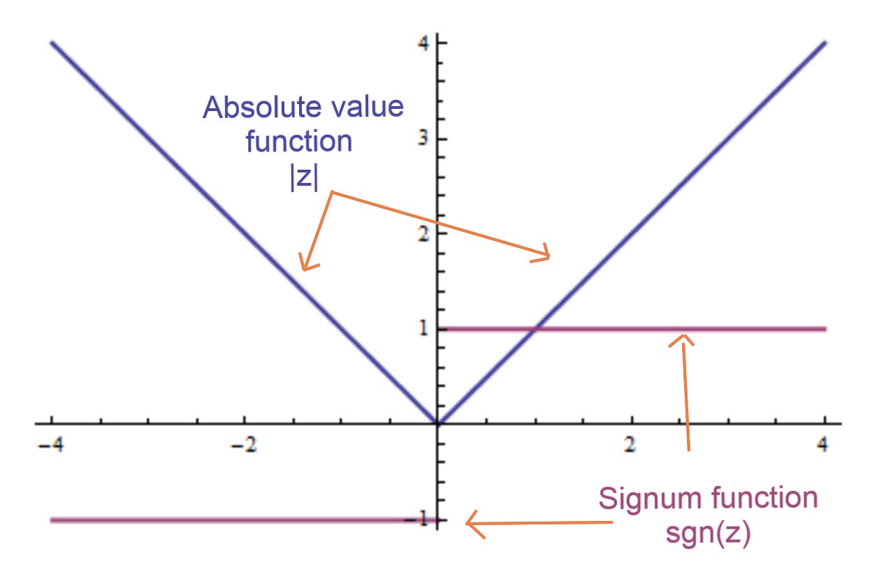
The signum/sign function (sgn)

Here the function sgn() is the derivation of absolute value function. It is also known as signum or sign function. Intuition behind this is very simple. If you differentiate the two sides (from z=0 axis) of the absolute value function, it would result in 1 with the sign of z as shown in the following figure. However the derivative at z=0 doesn’t exist. But here we don’t have to worry too much about that. You can find more information about the sgn() function in its wikipedia page.

For further discussions on how to join functions, here’s a Stackoverflow question.

Special thanks to Michal Fabinger (Tokyo Data Science) for explaining neural network essentials in a clear and concise way from where I obtained necessary the knowledge to compose this article.