In this story, we are going to discuss how probabilities and expected values work. You will figure out how to win at Roulette — at least in the short-term. If you’re looking for a way to become rich in the long-term, I have to disappoint you though. Sorry friend, this article is not for you.

But if you’re looking to understand probabilities and expected values for discrete random variables better — this is your story to read.

Let’s start by figuring out how Roulette works.

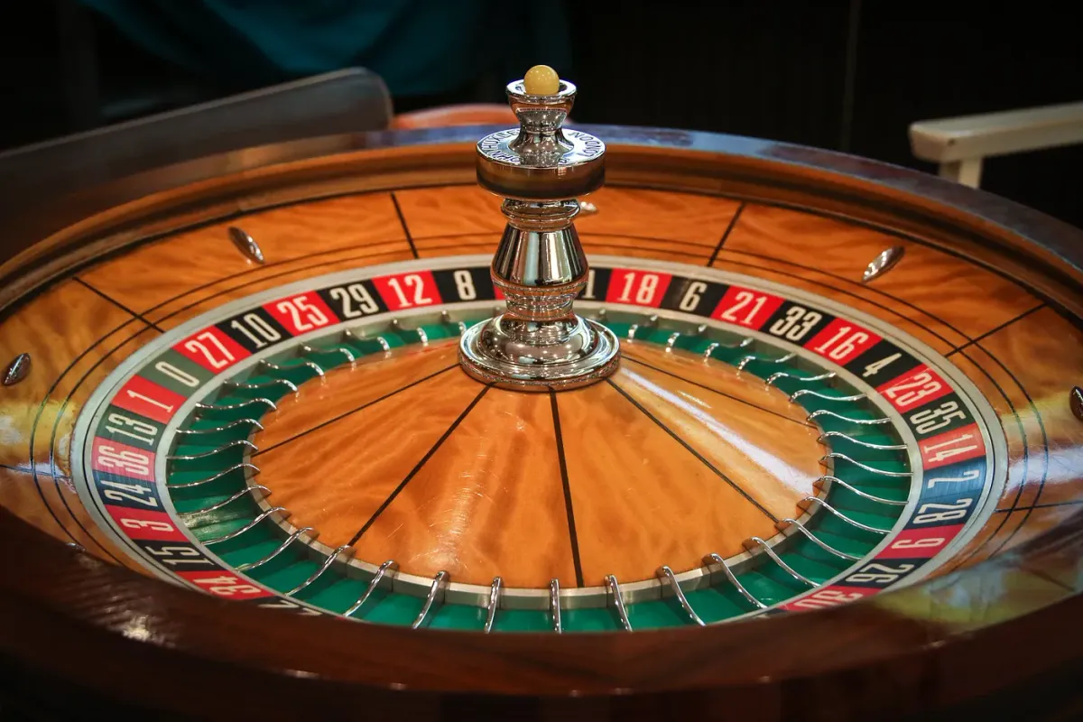
How does Roulette work?

Roulette is a wheel with 37 (European version) or 38 (American version) fields. A little ball is spun on the wheel until it lands on one of the 37 (European) or 38 (American) fields. The fields contain the numbers 0–36. In the American version, the zero exists twice. 18 of these fields without the zero are red and 18 are black, the zero (European version) or the zeros (American version) are usually green. The fields all have an equal chance to be drawn, players can bet on any combination of numbers, red or black, even or odd, high (numbers 19–36) or low (1–18).

In this story, we will only talk about the European version.

Basic Probabilities and Conditional Probabilities

In European Roulette, 37 fields may be hit. We call these 37 possible results Ω = {0, 1, 2, ….35, 36} our sample space. We can count the numbers of elements in Ω and it is, therefore, a discrete sample space. We can now calculate probabilities for subsets E of Ω, so-called events.

Ω: Sample Space

E ⊆ Ω: Event

Probabilities for such are calculated by dividing the number of elements in E by the number of elements in Ω.

Let’s define some events in Roulette, namely the events of a red number, a non-zero number and an odd number.

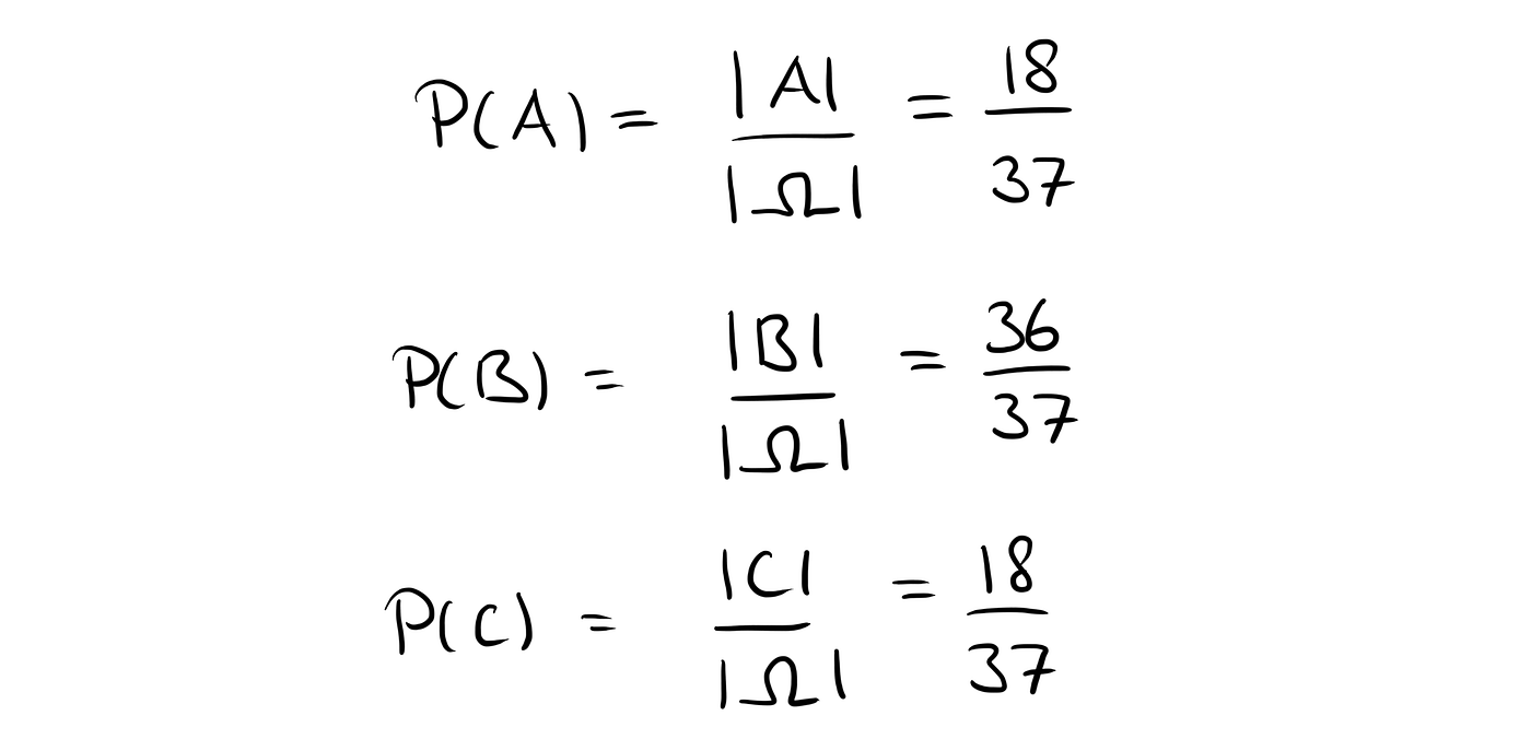
A = “Red” = {1, 3, 5, 7, 9, 12, 14, 16, 18, 19, 21, 23, 25, 27, 30, 32, 34, 36}

B = “Not Zero” = {1, 2, 3,…35, 36}

C = “Odd number” = {1, 3, 5, 7, …35}

We can then calculate these probabilities by dividing the number of elements in each event by the size of the sample space.

We can also calculate the probabilities of joint events. The joint event of two events A and B is the event that both A and B take place and it is denoted by A ∩ B. To determine this event, we can count or write down all the events that occur in both A and B. Since all elements in A are also in B, A ∩ B equals A. Of course, this does not happen in general and here it is due to how we defined A and B.

A ∩ B = “ Red and not zero” = “Red” = A

For A and C, the joint event A ∩ C is a little bit more interesting.

A ∩ C = “Red and Odd” = {1, 3, 5, 7, 9, 21, 23, 25, 27}

We can then calculate the probabilities as before by counting elements.

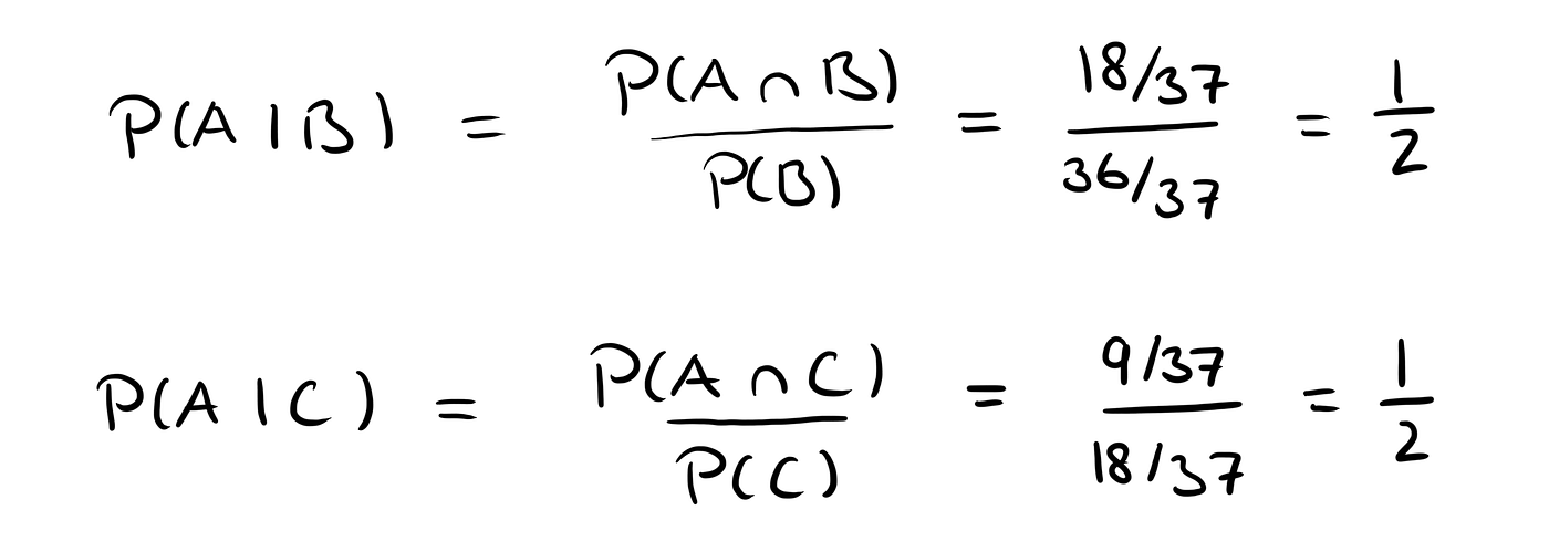
This now leads us to conditional probabilities. Conditional probabilities or the conditional probability of an event A given the event B is the probability of A given that B is already true. It basically means that we reduce our sample space to the new space B. The conditional probability is then given by

We can then calculate some of the conditional probabilities.

Now that we understand what probabilities and conditional probabilities are, we can move forward to expected values and conditional expectations.

Expected Values and Conditional Expectation

Expected values can be calculated for random variables. A random variable is a variable that takes real values and depends on chance. It is always denoted by a capital letter.

For example, we can bet 1$ on “Red” and define the random variable X.

The random variable X is then, for example, the amount of money won in this first bet.

X = amount of money won when betting 1$

X can take the values -1 (if we lose, i.e. “red” does not occur) or +1 if we win (i.e. red occurs). Once X has taken a value that we know (after the occurrence of the experiment, here spinning of the wheel), we write a small letter instead of a capital one.

The expected value is calculated by weighing all the possible outcomes (here 1 and -1) with the probabilities at which they occur and summing them all up.

Be careful here: The expected value is not really the value we would expect. Rather, it is the average value (weighted by the probabilities) that occurs. In fact, the expected value may never be observed. This is also the case here.

In our bet, the possible outcomes are -1 and 1 and they occur at a chance of 18/37 and 19/37 respectively.

Therefore we can calculate the expected value of X by

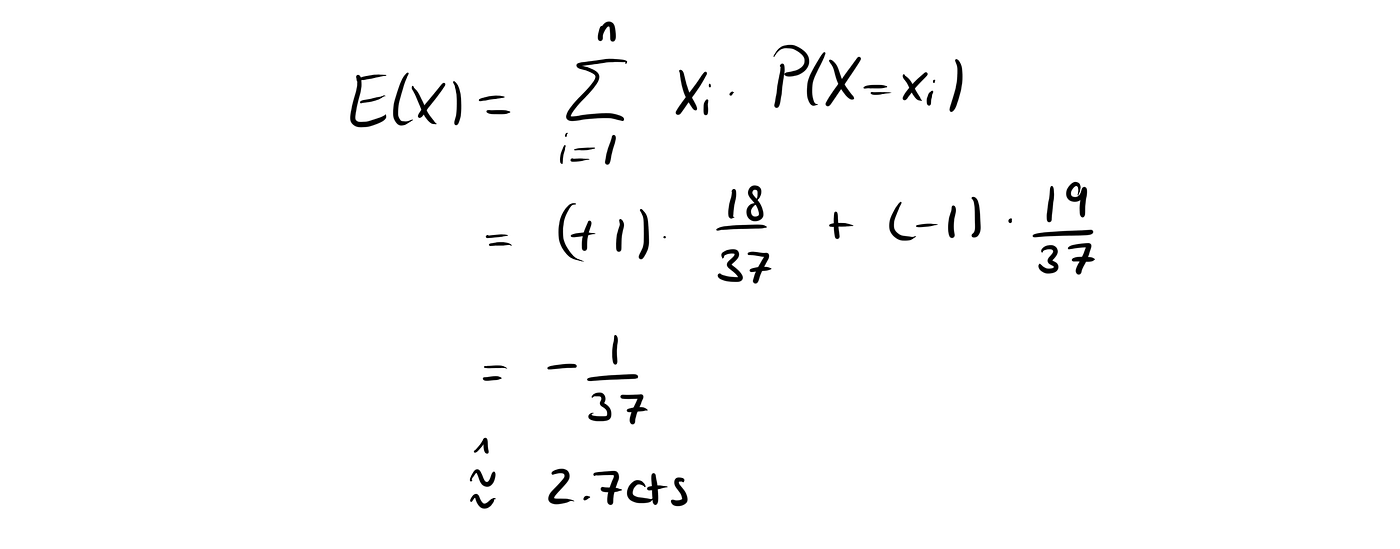
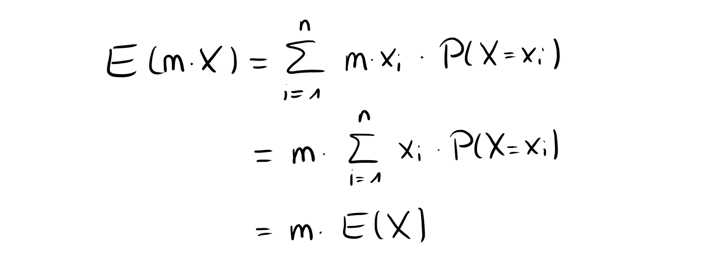
If we bet a different amount of money, say m, our expected value is then given by

This is the expected value. We can also define conditional probabilities and conditional expected values. For example let’s say that we already know that B occurred, i.e. that zero didn’t occur, but we don’t know anything else.

To calculate this expected value, we now use the conditional probabilities to calculate E(X|B).

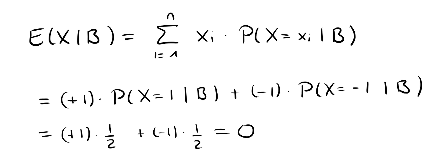
We call this game “fair Roulette” and the random variable X|B is the amount of money won when playing one round of fair Roulette.

We can also write

Stochastic Processes

So far, we have only looked at expected values and probabilities when playing once.

But people who go to casinos usually don’t just play once. They play multiple times and at the end of the day, it only matters how much money they have made in total.

To simulate this, we introduce stochastic processes. Stochastic processes are families of random variables X₀, X₁, X₂ and so on.

In our case, we define Xₙ for natural numbers n (including 0) by the amount of money won in the nᵗʰ game. Such a stochastic process is called a discrete-time stochastic process.

If we don’t play (as in the first game) we don’t win anything and we can define X₀ = 0.

A realization of the stochastic process is called a trajectory. For example,

is a possible trajectory for 7 games where we win, lose, lose, lose, lose, win and lose again and have always betted 1$.

The total amount of money won when always betting 1$ is then described by our stochastic process Y₀, Y₁, Y₂,… and a possible trajectory is then

We could now be interested in certain events, such as the chances of winning a certain amount of money or calculating expected values such as the expected win after playing 7 games.

But what we’re interested in is not calculating probabilities, but finding a strategy to win at Roulette.

For this, let’s calculate the expected value for the first game given that we know that our initial amount won is X₀ = 0.

So given that we have won nothing before our first game, our expected total win after the first game is E(X).

We can generalize this to the (n+1)ᵗʰ game, i.e. calculating our expected total win after n+1 games given that we know that after n games we have won yₙ.

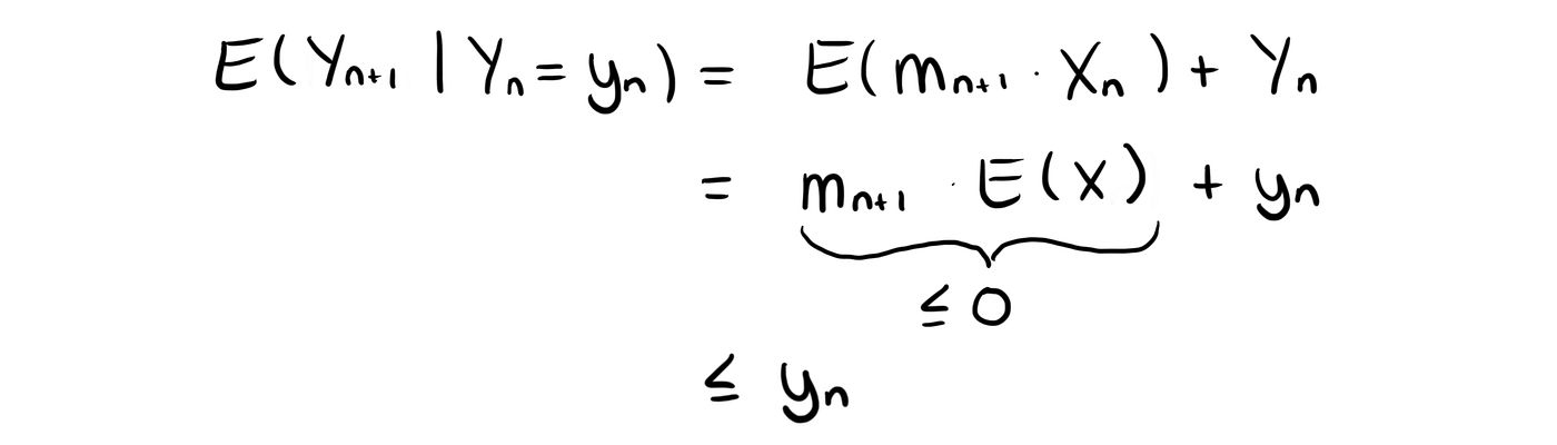
So the total expected amount won after the (n+1)ᵗʰ game given the total amount won after the nth game is whatever we have won after the nᵗʰ game plus the expected win for the (n+1)ᵗʰ game.

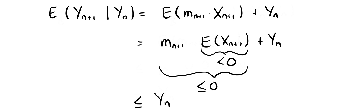
Now let’s assume we don’t know how much we have made after n games. Therefore, instead of writing Xₙ = xₙ we only write Xₙ and our conditional expectation

remains a random variable instead of a deterministic amount of money.

This leads us to the definition of martingales, sub-martingales, and super-martingales.

Martingales and Super-Martingales

A martingale is a stochastic process (Yₙ), n =1, 2, … for which holds

A super-martingale is a stochastic process for which holds

and a sub-martingale is a stochastic process for which holds

Also, in all cases,|Yₙ| needs to be finite for all n.

How can we interpret these stochastic processes? A martingale is a process for which the expected value at the next time step, given the current value of our process, is the same as our current process.

A series of games of fair Roulette where we always bet 1$ is such a martingale. Because the expected value of one game is 0, the expected value of our total win after the next game is our current win.

For the European Version of Roulette though, it is not a martingale. As we are expected to lose 2.7 cents when betting 1$ on Red, the expected total win after playing another game is our current win minus these 2.7 cents. So it’s less than our current win and thus the European (and American) Roulettes are both super-martingales.

They’re called super-martingales because they’re super (great) for the bank.

Unfortunately, not great for us.

If we had a sub-martingale though, this would be sub-optimal for the bank and super for us because in the next game we would be expected to make money instead of losing it (at least on average). Alternatively, if we find a strategy that has a total positive win (Yₙ >0) after some n, we would also be happy with a martingale.

Therefore, if we find a strategy that is a sub-martingale or such a positively valued martingale, we can, on average, win money.

The Martingale Strategy

We’re looking for a sub-martingale or a martingale and that’s why the strategy is called the Martingale Strategy.

And the idea is quite simple.

• We start by betting 1$.
• If we win, great. We have won 1 $. We stop playing (or we continue from the start)
• If we lose, we bet 2$. If we win, we win 2 $, thus making up for the first Dollar that we lost, winning 1$ in total. We stop.
• If we lose again, we bet 4$ next time. If we win, great. We just made up for the 1$+2$=3$ that we lost and won 1$ in total.
• If we lose again, we bet 8$ and continue the process always doubling the money we bet until we win. Then we stop and/or start from the beginning.

Why does this work? In the 0th bet, we bet nothing, i.e. m₀ = 0. In the first game, we bet 1$, i.e. m₁ = 1. For each game, we double this amount. Therefore, if we keep losing, in game number n, we bet mₙ = 2ⁿ⁻¹ Dollars.

Once we win, we stop betting money and start from time 0 again.

Let’s see what happens if we have our first win in game number 1, 2, 3, …n:

This means that if the first game in a series that we win is game number n₀, Yₙ will always be 1 after that (as we quit playing).

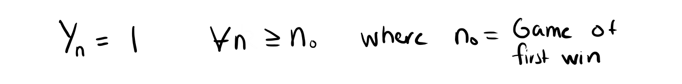
And therefore, for all n>n₀, our stochastic process will be a martingale, hence the name martingale strategy.

We will have one 1$ in this series.

Why you’re still going to lose money in the long run

The strategy sounds great, doesn’t it?

But I have to disappoint you. In the long run, you are always going to lose.

Why is that?

Because:

• You’re probably gonna have a losing streak at some point and go broke (the casino however never goes broke) because the money you have to bet doubles quite quickly (after 10 losses in a row you will already be at 1024$ in a single bet).
• Casinos usually have a betting limit, so at one point, you won’t be able to make up for your losses anymore.
• You will end up playing a lot of games just to make 1$ and you could be making so much more money doing something else or investing somewhere else.
• (And no, because of the betting limit it doesn’t work to simply start with 100$ instead of 1$).

So be wise, don’t gamble. Or do so, if you wish. But don’t blame me (or the math) for your losses.

About the Author: Maike is a coffee-fueled Mathematician who loves to teach, talk and write about Math. If you want to support her work, feel free to buy her a coffee: https://www.buymeacoffee.com/maikeelisa