Here we learn an ingenious application of a divide and conquer algorithm combined with linear algebra to multiply large numbers, fast. And an introduction to big-O notation!

In fact this result is so counter-intuitive that the great mathematician Kolmogorov conjectured an algorithm this fast did not exist.

Part 0: Long Multiplication is Slow Multiplication. (And an Introduction to Big-O Notation)

We all remember learning to multiply at school. In fact, I have a confession to make. Remember, this is a no judgement zone ;)

At school, we had ‘wet play’ when it was raining too hard to play in the playground. While other (normal/fun-loving/positive-adjective-of-choice) kids were playing games and messing about, I would sometimes get a sheet of paper and multiply large numbers together, just for the heck of it. The sheer joy of computation! We even had a multiplication competition, the ‘Super 144’ where we had to multiply a scrambled 12 by 12 grid of numbers (from 1 to 12) as fast as possible. I practised this religiously, to the extent that I had my own pre-prepared practice sheets which I photocopied, and then used on rotation. Eventually I got my time down to 2 minutes and 1 second, at which my physical limit of scribbling was reached.

Despite this obsession with multiplication, it never occurred to me that we could do it better. I spent so many hours multiplying, but I never tried to improve the algorithm.

Consider multiplying 103 by 222.

We calculate 2 times 3 times 1 +2 times 0 times 10 + 2 times 1 times 100 + 20 times 3 times 1 + 20 times 0 times 10 + 20 times 1 times 100 = 22800

In general, to multiply to n digit numbers, it takes O(n²) operations. The ‘big-O’ notation means that, if we were to graph the number of operations as a function of n, the n² term is really what matters. The shape is essentially quadratic.

Today we will fulfil all of our childhood dreams and improve on this algorithm. But first! Big-O awaits us.

Big-O

Look at the two graphs below

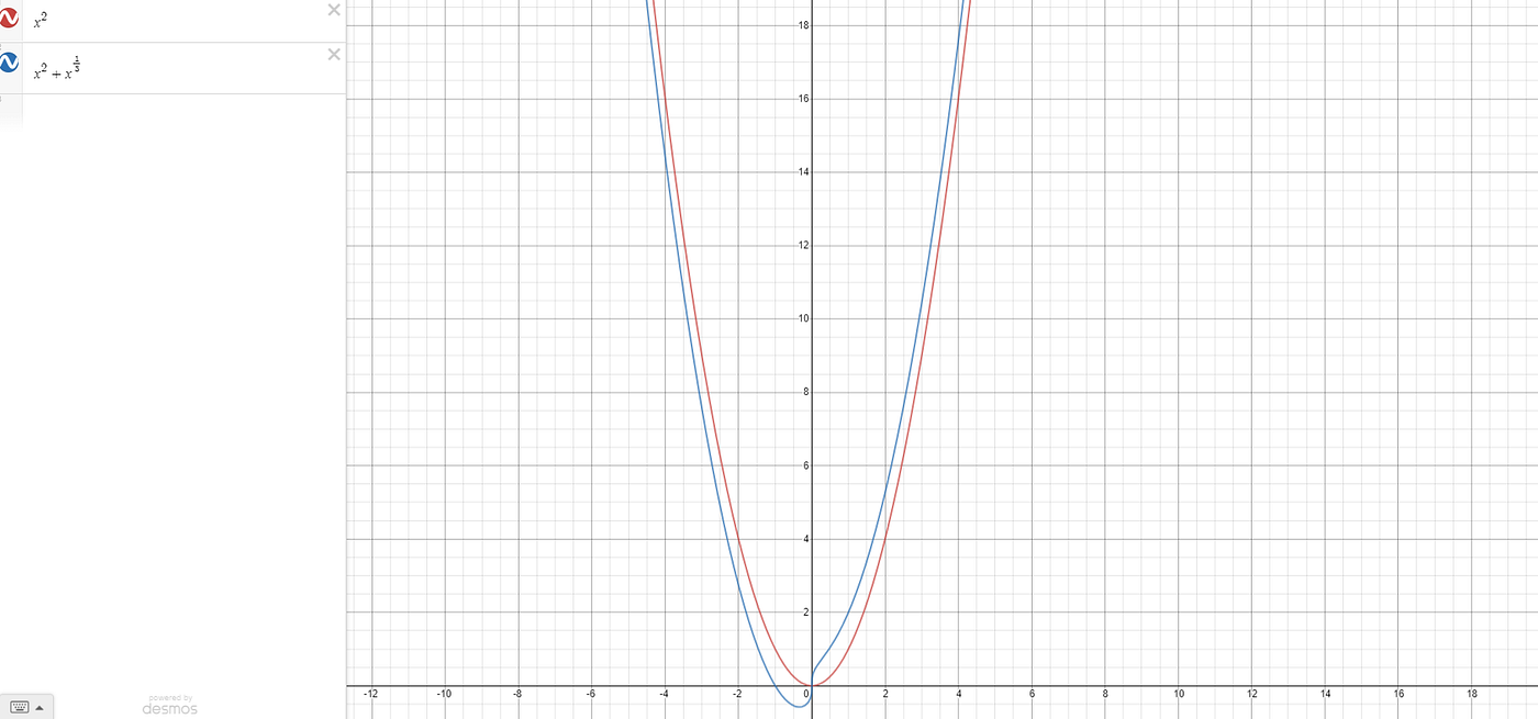
Ask a mathematician, “are x² and x²+x^(1/3) the same?”, and they will probably vomit into their coffee cup and start crying, and mumble something about topology. At least, that was my reaction (at first), and I scarcely know anything about topology.

Ok. They are not the same. But our computer doesn’t care about topology. Computers differ in performance in so many ways I can’t even describe because I know nothing about computers.

But there’s no point fine-tuning a steamroller. If two functions, for large values of their input, grow at the same order of magnitude, then for practical purposes that contains most of the relevant information.

In the graph above, we see that the two functions look pretty similar for large inputs. But likewise, x² and 2x² are similar — the latter is only twice as large as the former. At x = 100, one is 10,000 and one is 20,000. That means if we can compute one, we can probably compute the other. Whereas a function which grows exponentially, say 10^x, at x = 100 is already far far greater than the number of atoms in the universe. (10¹⁰⁰ >>>> 10⁸⁰ which is an estimate, the Eddington number, on the number of atoms in the universe according to my Googling*).

*actually, I used DuckDuckGo.

Part I: representing integers as Polynomials

Writing integers as polynomials is both very natural and very unnatural. Writing 1342 = 1000 + 300 + 40 + 2 is very natural. Writing 1342 = x³+3x²+4x + 2, where x = 10, is slightly odd.

In general, suppose we want to multiply two large numbers, written in base b, with n digits apiece. We write each n digit number as a polynomial. If we split the n digit number into r pieces, this polynomial has n/r terms.

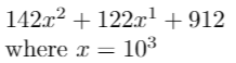
For instance, let b = 10, r = 3, and our number is 142,122,912

We can turn this into

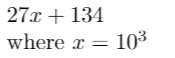
This works very nicely when r = 3 and our number, written in base 10, had 9 digits. If r doesn’t perfectly divide n, then we can just add some zeros at the front. Again, this is best illustrated by an example.

27134 = 27134 + 0*10⁵ = 027134, which we represent as

Why might this be helpful? To find the coefficients of the polynomial P, if the polynomial is order N, then by sampling it at N+1 points we can determine its coefficients.

For instance, if the polynomial x⁵ + 3x³ +4x-2, which is order 5, is sampled at 6 points, we can then work out the entire polynomial.

Intuitively, a polynomial of order 5 has 6 coefficients: the coefficient of 1, x, x², x³, x⁴, x⁵. Given 6 values and 6 unknowns, we can find out the values.

(If you know linear algebra, you can treat the different powers of x as linearly independent vectors, make a matrix to represent the information, invert the matrix, and voila)

Sampling polynomials to determine coefficients (Optional)

Here we look in a bit more depth at the logic behind sampling a polynomial to deduce its coefficients. Feel free to skip to the next section.

What we will show is that, if two polynomials of degree N agree on N+1 points, then they must be the same. I.e. N+1 points uniquely specify a polynomial of order N.

Consider a polynomial of order 2. This is of the form P(z) = az² +bz + c. By the fundamental theorem of algebra — shameless, plug here, I spent several months putting together a proof of this, and then writing it up, here — this polynomial can be factorised. That means we can write it as A(z-r)(z-w)

Note that at z = r, and at z = w, the polynomial evaluates to 0. We say w and r are roots of the polynomial.

Now we show that P(z) cannot have more than two roots. Suppose it had three roots, which we call w, r, s. We then factorise the polynomial. P(z) = A(z-r)(z-w). Then P(s) = A(s-r)(s-w). This does not equal 0, as multiplying non-zero numbers gives a non zero number. This is a contradiction because our original assumption was that s was a root of the polynomial P.

This argument can be applied to a polynomial of order N in an essentially identical way.

Now, suppose two polynomials P and Q of order N agree on N+1 points. Then, if they are different, P-Q is a polynomial of order N which is 0 at N+1 points. By the previous, this is impossible, as a polynomial of order N has at most N roots. Thus, our assumption must have been wrong, and if P and Q agree on N+1 points they are the same polynomial.

Part II: Divide and Conquer

Seeing is believing: A Worked Example

Let’s look at a really huge number which we call p. In base 10, p is 24 digits long (n=24), and we will split into 4 pieces (r=4). n/r = 24/4 = 6

p = 292,103,243,859,143,157,364,152.

And let the polynomial representing it be called P,

P(x) = 292,103 x³ + 243,859 x² +143,157 x+ 364,152

with P(10⁶) = p.

As the degree of this polynomial is 3, we can work out all the coefficients from sampling at 4 places. Let’s get a feel for what happens when we sample it at a few points.

• P(0) = 364,152
• P(1) = 1,043,271
• P(-1) = 172,751
• P(2) = 3,962,726

A striking thing is that these all have 6 or 7 digits. That’s compared with the 24 digits originally found in p.

Let’s multiply p by q. Let q = 124,153,913,241,143,634,899,130, and

Q(x) = 124,153 x³ + 913,241 x²+143,634 x + 899,130

Calculating t=pq could be horrible. But instead of doing it directly, we try to calculate the polynomial representation of t, which we label T. As P is a polynomial of order r-1=3, and Q is a polynomial of order r-1 = 3, T is a polynomial of order 2r-2 = 6.

T(10⁶) = t = pq

T(10⁶) = P(10⁶)Q(10⁶)

The trick is that we will work out the coefficients of T, rather than directly multiplying p and q together. Then, calculating T(1⁰⁶) is easy, because to multiply by 1⁰⁶ we just stick 6 zeros on the back. Summing up all the parts is also easy because addition is a very low cost action for computers to do.

To calculate T’s coefficients, we need to sample it at 2r-1 = 7 points, because it is a polynomial of order 6. We probably want to pick small integers, so we choose

• T(0)=P(0)Q(0)= 364,152*899,130
• T(1)=P(1)Q(1)= 1,043,271*2,080,158
• T(2)=P(2)Q(2)= 3,962,726*5,832,586
• T(-1)=P(-1)Q(-1)= 172751*1544584
• T(-2)=P(-2)Q(-2)= -1,283,550*3,271,602
• T(3)=P(-3)Q(-3)= –5,757,369*5,335,266

Note the size of P(-3), Q(-3), P(2), Q(2) etc… These are all numbers with approximately n/r = 24/4 = 6 digits. Some are 6 digits, some are 7. As n gets larger, this approximation gets more and more reasonable.

So far we have reduced the problem to the following steps, or algorithm:

(1) First calculate P(0), Q(0), P(1), Q(1), etc (low cost action)

(2) To get our 2r-1= 7 values of T(x), we must now multiply 2r-1 numbers of approximate size n/r digits long. Namely, we must calculate P(0)Q(0), P(1)Q(1), P(-1)Q(-1), etc. (High cost action)

(3) Reconstruct T(x) from our data points. (Low cost action: but will come into consideration later).

(4) With our reconstructed T(x), evaluate T(10⁶) in this case [T(b^(n/r)) in general for base b and length n]

This nicely leads to an analysis of the running time of this approach.

Running time

From the above, we found out that, temporarily ignoring the low cost actions (1) and (3), the cost of multiplying two n digit numbers with Toom’s algorithm will obey:

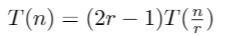
This is what we saw in the worked example. To multiply each P(0)Q(0), P(1)Q(1), etc costs T(n/r) because we are multiplying two numbers of length approximately n/r. We have to do this 2r-1 times, as we want to sample T(x) — being a polynomial of order 2r-2 — at 2r-1 places.

How fast is this? We can solve this sort of equation explicitly.

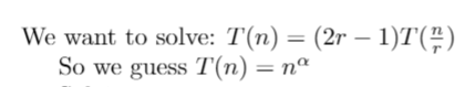
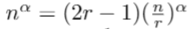
All that remains now is some messy algebra

As there were some other costs from the matrix multiplication (‘reassembling’) process, and from the addition, we cannot really say that our solution is the exact runtime, so instead we conclude that we have found the big-O of the runtime

Optimising r

This runtime still depends on r. Fix r, and we are done. But our curiosity is not yet satisfied!

As n gets large, we want to find an approximately optimal value for our choice of r. I.e. we want to pick a value of r which changes for different values of n.

The key thing here is that, with r varying, we need to pay some attention to the reassembly cost — the matrix which performs this operation has a cost of O(r²). When r was fixed, we didn’t have to look at that, because as n grew large with r fixed, it was the terms involving n which determined the growth in how much computation was required. As our optimal choice of r will get larger as n gets larger, we can no longer ignore this.

This distinction is crucial. Initially our analysis chose a value of r, perhaps 3, perhaps 3 billion, and then looked at the big-O size as n grew arbitrarily large. Now, we look at the behaviour as n grows arbitrarily large and r grows with n at some rate we determine. This change of perspective looks at O(r²) as a variable, whereas when r was kept fixed, O(r²) was a constant, albeit one we didn’t know.

So, we update our analysis from before:

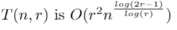
where the O(r²) represents the cost of the reassembly matrix. We now want to choose a value of r for every value of n, which approximately minimises this expression. To minimise, we first try differentiating with respect to r. This gives the somewhat heinous looking expression

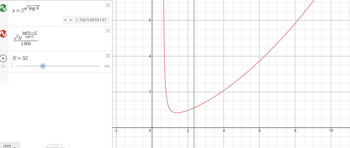
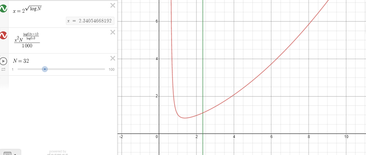
Normally, to find the minimum point, we set the derivative equal to 0. But this expression doesn’t have a nice minimum. Instead, we find a ‘good enough’ solution. We use r = r^(sqrt(logN)) as our guestimate value. Graphically, this is pretty near the minimum. (In the diagram below, the 1/1000 factor is there to make the graph visible at reasonable scale)

The graph below shows our function for T(N), scaled by a constant, in red. The green line is at x = 2^sqrt(logN) which was our guestimate value. ‘x’ takes the place of ‘r’, and in each of the three pictures, a different value of N is used.

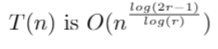
This is pretty convincing to me that our choice was a good one. With this choice of r, we can plug it in and see how our algorithm’s final big-O:

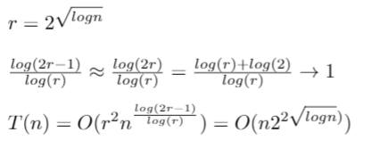
where we simply plugged in our value for r, and used an approximation for log(2r-1)/log(r) which is very accurate for large values of r.

How Much of An Improvement?

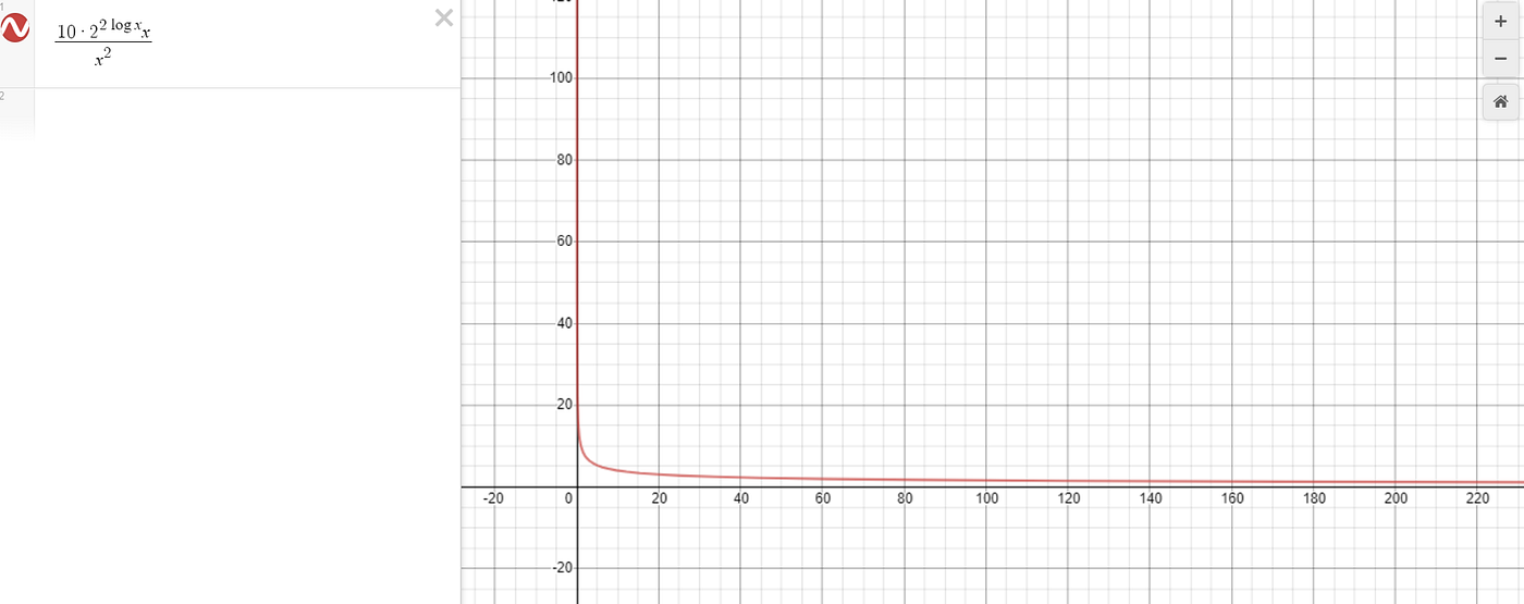
Perhaps me not spotting this algorithm when I was a wee lad doing multiplication was reasonable. In the graph below, I give the coefficient of our big-O function to be 10 (for demonstration purposes) and divide it by x² (as the original approach to multiplication was O(n²). If the red line tends to 0, that would show our new running time asymptotically does better than O(n²).

And indeed, while the shape of the function shows that our approach is eventually faster, and eventually it is much faster, we have to wait until we have nearly 400 digit long numbers for this to be the case! Even if the coefficient was just 5, the numbers would have to be about 50 digits long to see a speed improvement.

For my 10 year old self, multiplying 400 digit numbers would be a bit of a stretch! Keeping track of the various recursive calls of my function would also be somewhat daunting. But for a computer doing a task in AI or in physics, this is a common problem!

How profound is this result?

What I love about this technique is that it is not rocket science. It’s not the most mind-boggling mathematics every to be discovered. In hindsight, perhaps it appears obvious!

Yet, this is the brilliance and beauty of mathematics. I read that Kolmogorov conjectured in a seminar that multiplication was fundamentally O(n²). Kolmogorov basically invented lots of modern probability theory and analysis. He was one of the mathematical greats of the 20th century. Yet when it came to this unrelated field, it turned out there was an entire corpus of knowledge waiting to be discovered, sitting right under his and everyone else’s noses!

In fact, Divide and Conquer algorithms spring to mind fairly quickly today as they are so commonly used. But they are a product of the computer revolution, in that it is only with vast computation power that human minds have been focusing specifically on the speed of computation as an area of mathematics worthy of study in its own right.

This is why mathematicians aren’t just willing to accept the Riemann Hypothesis is true just because it seems like it might be true, or that P does not equal NP just because that seems most likely. The wonderful world of mathematics always retains an ability to confound our expectations.

In fact, you can find even faster ways to multiply. The current best approaches use fast fourier transforms. But I’ll save that for another day :)

Let me know your thoughts down below. I am newly on Twitter as ethan_the_mathmo, you can follow me here.

I came across this problem in a wonderful book I am using called ‘The Nature of Computation’ by Physicists Moore and Mertens, where one of the problems guides you through analysing Toom’s algorithm.