How do Scientists Formulate New Equations?

This question must have crossed your mind at least once, even though you may not be so much of a fan of mathematics. If you are a curious person with a genuine interest, it even gets worse — or better for that matter. As for me, this question lingered in my mind for over 19 years and I only got an idea after completing my graduate studies. If you have never thought about this topic critically, and you intend to pursue a Ph.D. at some point, especially in any STEM field, it’s time you started developing interest. This is a necessity, at least if you want your life to be easier during this important period of your life.

Where there is a number, there is beauty — Proclus

So how the heck did Albert Einstein come up with the equation E = mc², or how did Isaac Newton found F=ma for instance? Well, while I do not claim to be of the same calibre as renowned scientists who have been successful in corroborating these kind of equations, I will share a few tips that may guide you towards understanding just a bit of how such equations emerge.

You will be surprised how easily equations can be formed from ab initio — or from first principles, especially if you have some prior information about the physical system you are trying to model or represent in the language of mathematics. There is one example that I like to use when I try to explain this topic to someone who has gone through high school mathematics, and passed at least one course in calculus, and I will repeat here. As a matter of fact, let’s wrap it all up into the concept’s acronym: RADICAL, to mean Regression Analysis, DImensional Analysis, and CALculus — no pun intended, but those are the methods you will want to acquaint yourself with in order to perfectly understand what we will discuss. You don’t need to go deep in each, but just know what they are.

Equation(s) of Linear Motion

Let’s start with some of the simplest cases of rectilinear motion, aka linear motion. So, supposing you come in contact with an intelligent alien from another planet. This alien only understands the dimensions of all our physical units, but does not know how we conduct our maths, for instance, it knows that displacement or distance, s is somehow related, or is a function of velocity or speed, v, and velocity is in turn, a function of time, t. Unfortunately, it does not know the exact relationship for estimating the velocity of a moving object like we do. We know for instance, within a given time, the speed is given by the formula:

With the first term on the Right hand Side (RHS) being the initial velocity, and the second is a multiple of acceleration, a with time. This information is not accessible to the Alien. How would the Alien come up with the above formula, is the question we also ask ourselves in this situation. So mathematically (as aliens), we would start by representing the given information in terms of two other functions f and g, such that:

This allows us to write the derivative of distance, s in form of differentials as follows:

What did we just do? We have expressed the first part of Eq. (2) in differentials form. Meaning that a small change in the displacement, s is directly proportional to its partial derivative with respect to the speed, v. The constant of proportionality is the delta — counterpart of s. We then do the same for the second function in Eq. (2), and now take the limits as that small division (delta) tend towards zero to get the following forms:

As you can see, our equation is now starting to look familiar. Now, let us introduce regression and dimensional analysis at the same time. That means we look at the units of the both sides to determine what the heck is going on. The left hand side (LHS) is just units of length, L divided by that of time, T. Following that routine, we can re-write the whole of Eq. (4) as follows:

Where the beta terms are nothing but regression coefficients. Of course we are curious to find out what the coefficients really are, and the answer is dimensional analysis. The units on the LHS must be the same as those on the RHS, and thus β_0 must have the units of speed, m/s and β_1 must be determined by division — this gives seconds or simply s and we are done. We now just need to set the β coefficients and write the final equation as follows:

Notice that we didn’t have to know this final form, but we managed in the end to re-write it. Finally, you may want to roll back and find the formula for instantaneous distance, s. This simply means re-writing s, but this time as a continuous function of time, which is achieved by integrating Eq.(6) with respect to time. That will lead to one of the most familiar forms in which equations of linear motion are usually presented being, s = 1/2 at². As a side note, did you know that the regression coefficients are also the partial derivatives of that function with respect to the variables they represent? Here is another example:

Derivation of Newton’s First Law

So supposing over your studies you have noticed that the momentum, P of an object, say a stone rolling down a hill is a function of its mass and its velocity, but you don’t know for sure that P=mv — this is the final form we want to achieve.You will then follow the same routine to arrive at the statement that:

If P is a function of m and v and both m and v are functions of another variable t , then Pmust also be a function of t.

As a matter of fact, there is a more common name for converting such statements into mathematical formulae. It is referred to as the Chain rule. Without even needing to write the differentials, you can immediately write the following:

Then you proceed to the next step, which is the regression analysis. It gets even better if you are used to some rules of calculus, in this case the product rule of differentiation will immediately give you the relationship between P, m and v, in that momentum must be given as: P = mv. As you can see, just by expressing the given variables as functions, you can land onto the answer. The problem is of course at that moment you are oblivious of the form you are looking for since we are assuming a complete start, with no prior knowledge of the equation you are looking for. We are therefore assuming that once you end up with a promising form, you proceed to perform the experiments. In that way, you not only reduce the cost of experimentation, but you also accelerate your working progress, and thereby reducing the time spent on the project in general.

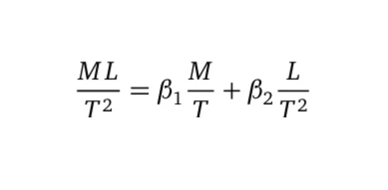
Replace the partial derivatives with β coefficients and proceed to dimensional analysis. You will realize that the LHS is nothing but force, F. That means, in all we do, the RHS must also yield the units equivalent to those of force i.e. kgm/s². So we update Eq. (7) as follows:

You can then easily tell the units of each β coefficient by applying the rule that the units on both sides must match. The first coefficient must have units of velocity, while that of the second one must be mass, and thus the semi final form can be written as follows:

Above system represents Newton’s first law of motion, when change in mass is taken into consideration. This is normally the case when you are trying to represent a system where the mass reduces or increases as the object moves, for example a rolling ball of glacier or snow down the hill. It could be gathering more mass or breaking loose, and thus you would adjust the signs in Eq. (9) appropriately. I would have likened it to the rocket as the fuel tanks are jettisoned when they run empty, but this is an overkill that might scare most readers off.

So let’s stick to snow, glaciers or stones being the objects that we all know of and can relate to. In the event that no change in mass is involved, Eq. (9) simplifies further to the very form most of us are aware of, F = ma. That means you ignore the term with dm/dt by setting it to zero, and replacing dv/dt by the derivative of Eq. (6) with respect to time.

Now, as a concluding remark I may not have created a new equation here, but it is possible and I am claiming that having have had to create one or two entirely new equations in the past when it was completely necessary. I encourage you to try this in your everyday life and you will gain abundance of nuances. There is an underlying beauty in mathematics that can both be surprising and blissful at the same time. Perhaps it’s true that where there is a number, there is beauty — Proclus