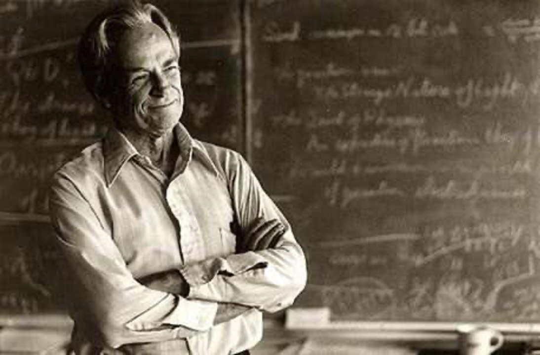
The American theoretical physicist Richard Feynman is one of the best-known scientists in the world (see this link). Feynman made several contributions to theoretical physics. These include: a new formulation of quantum mechanics using path integrals, the theory of quantum electrodynamics (including the development of his famous pictorial representations known as Feynman diagrams), his contributions to the explanation of the phenomenon of superfluidity of supercooled liquid helium, and his pioneering work in quantum computing and nanotechnology. In 1965, he was one of the recipients of the Nobel Prize in Physics.

In his biography about Feynman, the American-Canadian theoretical physicist Lawrence Krauss attributes the following quote to him:

“There is pleasure in recognizing old things from a new viewpoint.”

— Richard Feynman

In this article, based on Sakurai, I will introduce Feynman’s brilliant new approach to quantum theory, based on path integrals.

Old Approaches to Quantum Mechanics

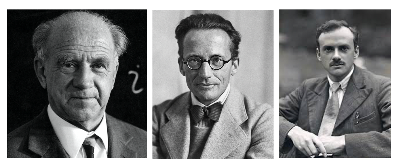
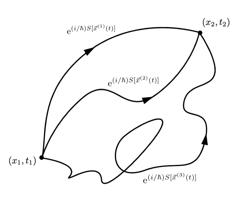
The first successful attempt to replicate the quantization of the atomic spectra was called matrix mechanics. It was developed in 1925 by the German theoretical physicist Werner Heisenberg. In the same year, the Austrian-Irish physicist Erwin Schrödinger created his wave mechanics. After a year, Schrödinger himself proved the equivalence of both approaches. However, the modern view of quantum mechanics, where states are mathematical entities in Hilbert space, is attributed mainly to the English theoretical physicist Paul Dirac. Driven by the development of quantum field theory, other formulations of quantum mechanics were developed.

One of these approaches was the path integral formulation, which is a generalization of the action principle of classical mechanics. In this formalism, the quantum transition between two states is obtained by “summing” (more precisely evaluating a functional integral) over all possible classical trajectories. This formulation, therefore, replaces the classical notion that a single spacetime trajectory is associated with the motion of a system. Though the development of the path integral formulation involved other scientists (such as Norbert Wiener and Paul Dirac), the complete method was provided by Feynman in 1948.

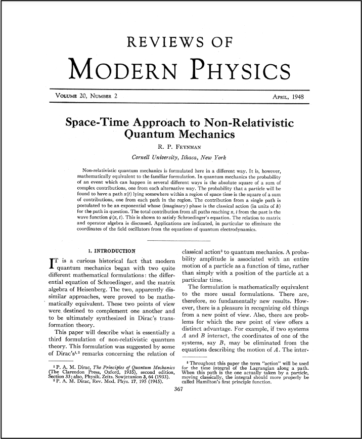
The abstract of the article “Space-Time Approach to Non-Relativistic Quantum Mechanics”, where Feynman introduced his new approach reads:

“[Q]uantum mechanics is formulated here in a different way. It is, however, mathematically equivalent to the familiar formulation. In quantum mechanics the probability of an event which can happen in several different ways is the absolute square of a sum of complex contributions, one from each alternative way. The probability that a particle will be found to have a path x(t) lying somewhere within a region of spacetime is the square of a sum of contributions, one from each path in the region. The contribution from a single path is postulated to be an exponential whose (imaginary) phase is the classical action (in units of h/2π) for the path in question. The total contribution from all paths reaching x, t from the past is the wave function ψ(x, t). This is shown to satisfy Schrödinger’s equation...”

To start, I will first introduce the concept of a quantum propagator.

Quantum Propagators

Propagators in quantum mechanics and quantum field theory are functions that determine the probability amplitude for a particle to move from one position to another in a given interval of time (transition amplitude). The modulus squared of the transition amplitude is the transition probability.

Let the time-dependent X(t) be the position operator in the Heisenberg picture. Using the elegant (bra and ket) notation developed by Dirac, consider the following initial and final vector states

which are eigenstates of the operator X(t):

The propagator corresponding to the transition in Eq. 1 is given by the following expression:

This function (the propagator) is a transition amplitude.

Completeness of the Set of Position Kets

Naturally, the probability that we get any result when we measure the position of a system (at some fixed time) must be equal to 1. A consequence of this is that position kets form a complete set:

Note that the unit on the right-hand side is the identity operator. This relation can be used to write the propagator as a succession of integrals. In other words, we can write a transition as a combination of intermediary transitions. The simplest case is:

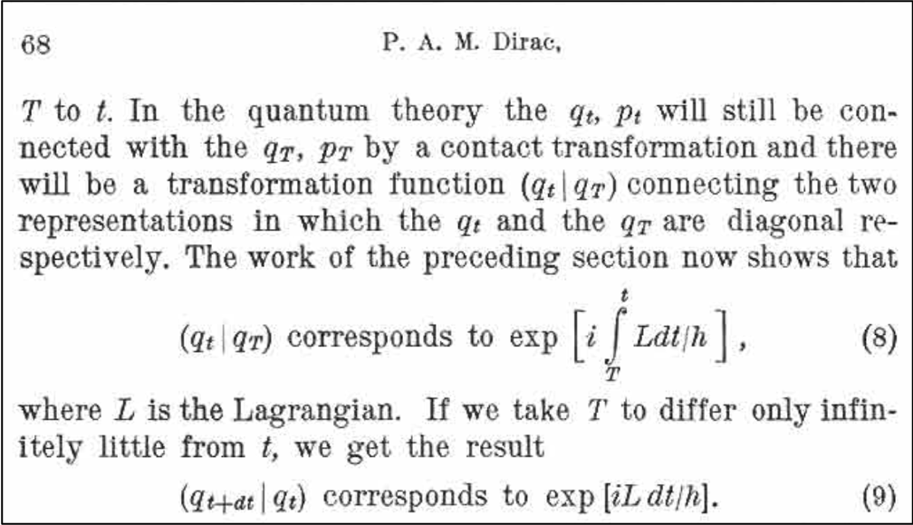
Using this compositional property of the propagator we may divide the time interval corresponding to a transition between two states

into equal parts with the length

and then write the transition amplitude as a composition of amplitudes:

We are summing over all possible paths, with fixed endpoints. This is illustrated in the middle plot in Fig. 4.

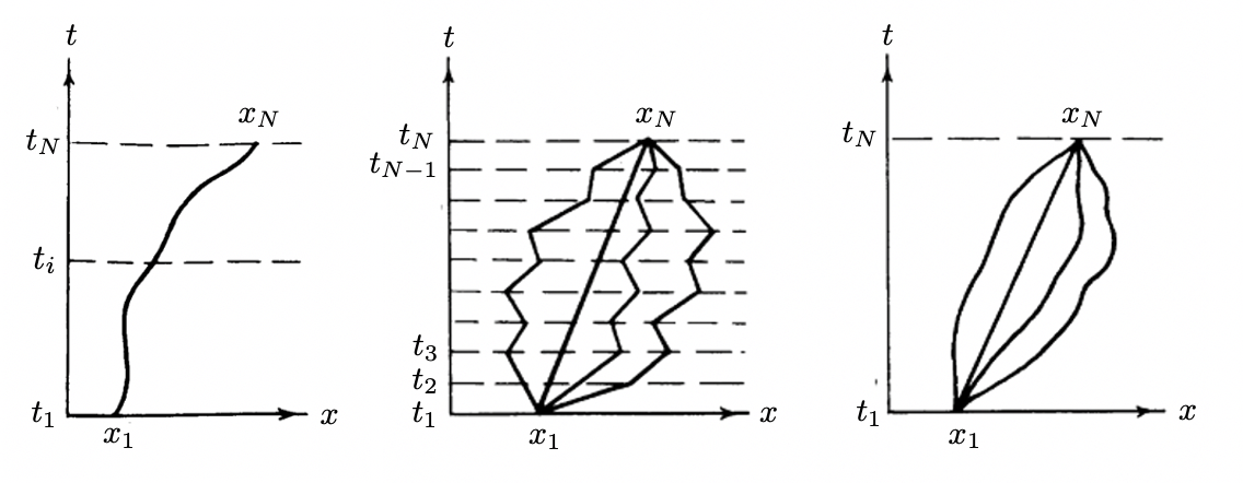
The leftmost plot in Fig. 4 shows the classical mechanics' unique path. To obtain this path consider a particle with an associated Lagrangian L(x, dx/dt). The Lagrangian equation of motion, which describes the path, is obtained by extremizing the action:

This is called the Hamilton principle.

Feynman’s Space-Time Approach

As we just saw, while in classical physics a particle motion has a definite path, in quantum mechanics all possible paths must be taken into account. The question is: in the limit h→ 0 how can we show that quantum mechanics reproduces classical mechanics?

In a 1933 paper, Paul Dirac made a mysterious remark which puzzled Feynman. Adapting the notation (following Sakurai), the statement was:

Feynman was troubled with the meaning of Dirac’s remark. What did he mean by “corresponds to”? This questioning led Feynman to the formulation of his powerful space-time approach to quantum mechanics.

Following Sakurai, the action corresponding to a small segment of the path reads:

For a given path, we obtain the corresponding amplitude by multiplying such expressions. The propagator for the transition in Eq. 5 is then obtained by a sum over all paths:

For small h, the only relevant term of this sum corresponds to a path that does not vary if we deform it slightly (since h is small, the contribution of the other paths cancel out due to the strong oscillation of the exponentials). This means that this path satisfies Eq. 8:

Therefore, according to Hamilton’s principle, the amplitude depends only on the classical path (more precisely, on a narrow strip that contains the classical path). Hence classical mechanics is recovered for small h, as it should!

Feynman rewrote Dirac’s Eq. 11 as a proportionality:

In his biography about Feynman, James Gleick describes the following conversation between the two great men:

“Feynman looked out the window and saw Dirac... He had a question that he had wanted to ask Dirac since before the war. He wandered out and sat down. A remark in a 1933 paper of Dirac’s had given Feynman a crucial clue toward his discovery of a quantum-mechanical version of the action in classical mechanics [see Eq. 9 above]. Dirac had written, but neither he nor anyone else had pursued this clue until Feynman discovered that the “[corresponds]” was, in fact, exactly proportional. There was a rigorous and potentially useful bond. Now, he asked Dirac whether the great man had known all along that the two quantities were proportional. “Are they?” Dirac said. Feynman said yes, they were. After a silence Dirac walked away.”

Setting V=0 for simplicity, using a linear approximation for S(n, n-1) and integrating both sides of Eq. 13, one quickly obtains the prefactor 1/w(Δt):

The transition amplitude for the full path is obtained by integrating over all intermediate steps:

where:

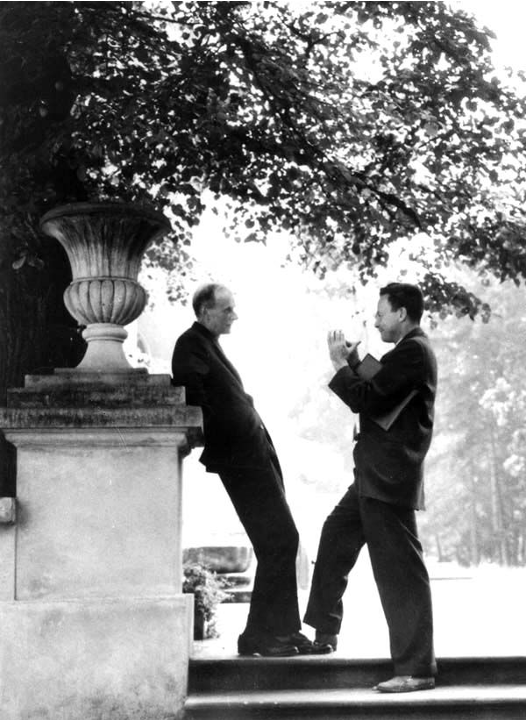
This is the so-called Feynman’s path integral and is the sum (or integral) of all possible paths. The corresponding diagram is shown in Fig. 4 (third plot) and Fig. 6.

Note here that in contrast to the other formulations of quantum mechanics, the probability amplitude is not a linear complex superposition of quantum states. It is a quantum superposition of entire alternative space-time histories (between fixed points). The idea here is that quantum mechanically there is a complex superposition of “alternative realities” (alternative histories). However, the exponential weighting, usually called amplitude,

is, in fact, an “amplitude density” since there is a continuous infinity of classical alternatives and we must therefore integrate over the space of classical paths. Since we have infinite classical paths, this space is infinite-dimensional and the integral is known to have pathological behavior.

Also, it should be noted that the trajectories do not need to obey the rules of special relativity: any trajectory is possible provided the endpoints are fixed (see figure below). Fig. 8 below illustrates the case of a single particle.

Equivalence of Feynman’s and Schrödinger’s Approach: A Proof

We shall now prove that Feynman’s approach is equivalent to Schrödinger wave mechanics. We start by writing:

where we assumed:

We now rename the final position and final time as x and t + Δt, use ξ in Eq. 18, and expand the exponential and the amplitude (inside the integral) in powers of ξ. Collecting terms and performing trivial Gaussian integrals we obtain:

We conclude that Feynman’s propagator and Schrödinger’s propagator (obtained using his wave mechanics) are the same objects!

Thanks for reading and see you soon! As always, constructive criticism and feedback are always welcome!

My Linkedin, personal website www.marcotavora.me, and Github have some other interesting content about physics and other topics such as mathematics, machine learning, deep learning, finance, and much more! Check them out!