How Does Compression Work?

I structured this article in a way that you are gonna need your focus at the first section when I explain about the SVD decomposition and just after that you’ll get your reward which will be watching how it works in a full demo.

Before we begin, note that I’m going to assume you know what matrices and eigenvalues are.

Definitions & Assumptions

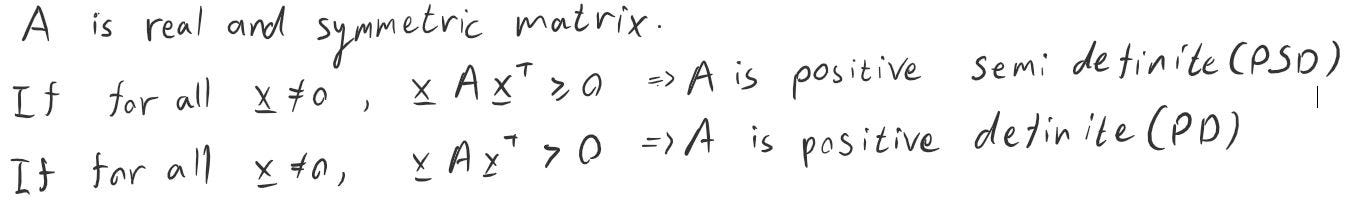
A thing you should remember is if A is PSD then all its eigenvalues are greater or equal to zero, and as you have probably guessed — if A is PD all its eigenvalues are greater than zero.

Another important fact about the PSD matrices is

Note that this fact is also true for A*Aᵀ (simply substitute Aᵀ with A).

Before we continue, just to make sure we are on the same page, I will denote the matrix ‘A transpose’ with Aᵀ and throughout this article I won’t regard to the case of complex matrices so we won’t need the conjugate transpose.

Note that if A had n rows and m columns, A * Aᵀ will have n rows and n columns, meaning that A* Aᵀ is always a square matrix.

We are really close to the SVD decomposition, but we will have to go through singular values before we jump into that.
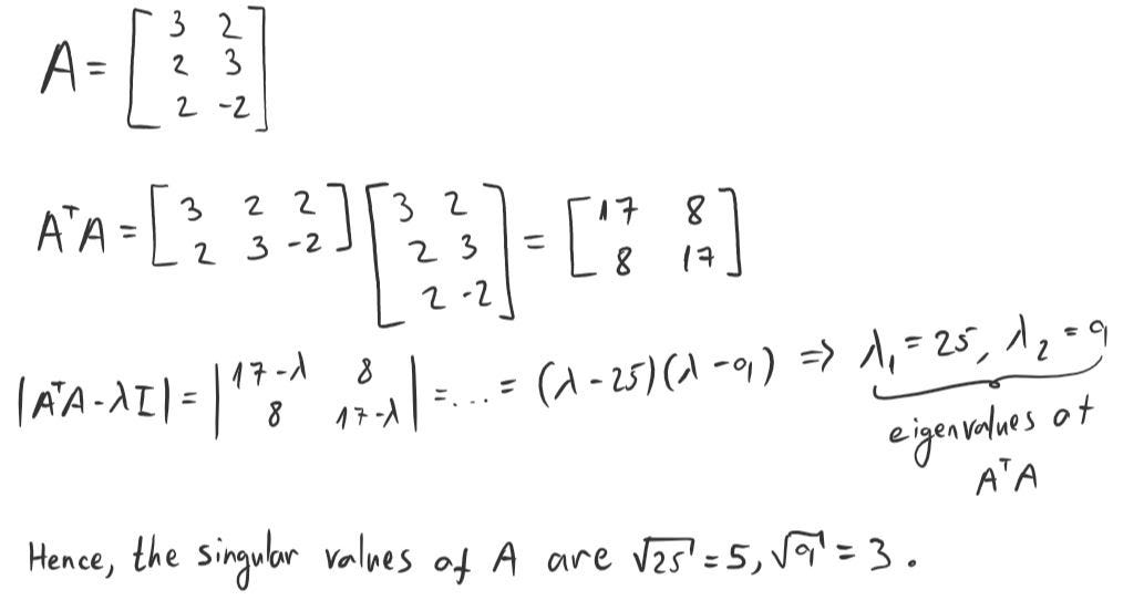
In short, the singular values of matrix A are the square roots of eigenvalues of matrix A * Aᵀ.

In case the above wasn’t so clear, here’s an example

SVD Decomposition

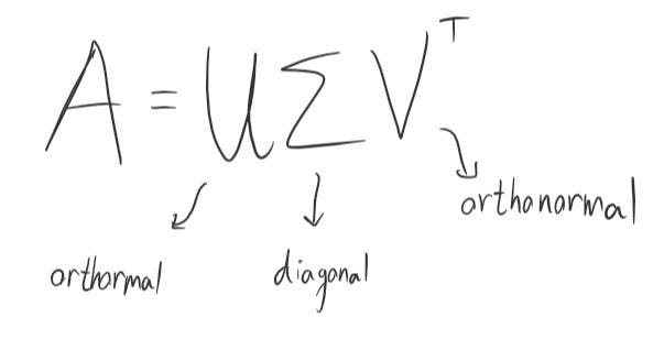
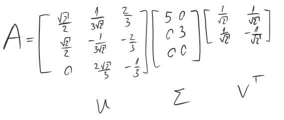
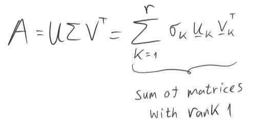
Every real matrix A with m rows and n columns can be decomposed into U*Sigma*Vᵀ
When U is orthonormal with m rows and columns;
V^T is orthonormal with n rows and columns;
And Sigma is a diagonal matrix with m rows and n columns.

In order to get the SVD decomposition of a matrix we will need to follow 6 steps.

• Calculate Aᵀ * A.
• Find the eigenvalues and eigenvector of this matrix (if eigenvectors aren’t orthonormal — use gram schmidt process).
• Collect the eigenvectors from the previous step and plug them in as rows of Vᵀ.
• Take the square root out of the eigenvalues and plug them in S(sigma) diagonal.
• Calculate u=Av, normalize them then plug them in as U columns.
• In case U is not a square matrix, use the gram schmidt process to generate more orthonormal vectors.

I will continue with the previous example completing all the above steps.
We have done step 1 and half of step 2 so far, here are the eigenvectors of Aᵀ *A.

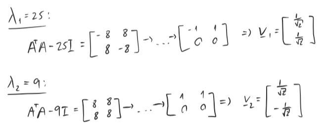
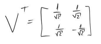
Moving on to step 3, we will just take both the vectors we have found above and plug them in Vᵀ rows

Next, another easy step ahead of us but bear in mind that Sigma needs to be of the same size of A.

Another important thing I haven’t discussed before is that the singular values needs to be on the diagonal on descending order so it’s crucial that in this case Sigma is just as I wrote it (bottom version of course).

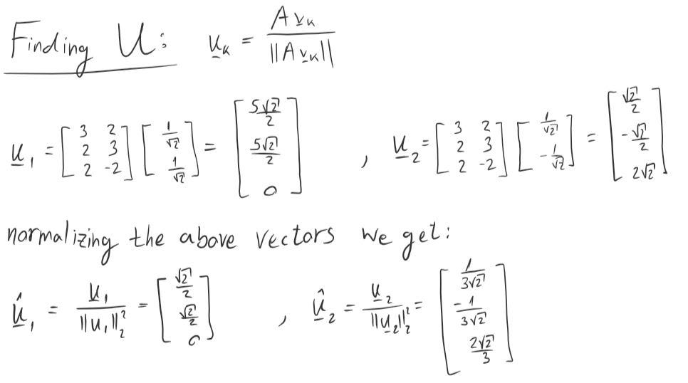
Moving on to the next step, we are searching this time for U columns.
Remember that U needs to be of size mxm and we only have to eigenvectors so that means we will have to find another orthonormal vectors afterwards on step 6.

In order to find a third vector which will be orthonormal to the other two vectors we have just found we can either use the Gram-Schmidt process or just make some equations that represent our demands

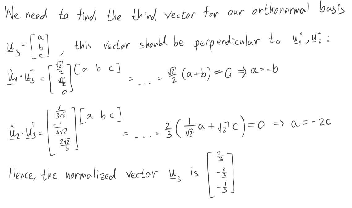
Finally, we got our SVD decomposition

How can we use SVD decomposition to compress images

To answer this answer we first have to tackle the following question.
Given matrix A (of rank m), what is the closest matrix B (of rank r < m) to A?

Let’s break this problem down by first understanding how do we measure distance between matrices.

There is more than one way to measure this distance, I chose to use the Frobenius Norm which is practically similar to the L2 norm for vectors if you flaten your matrix into a 1D vector.

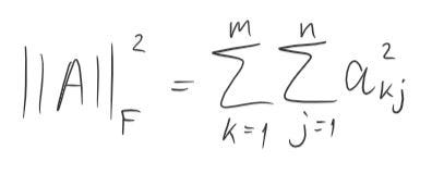
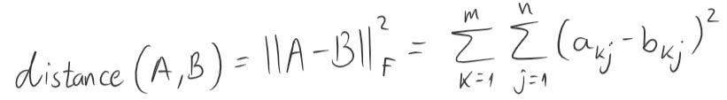
We will define distance between matrices as the Frobenius Norm of the subtraction between them.

Then we can rephrase our problem to

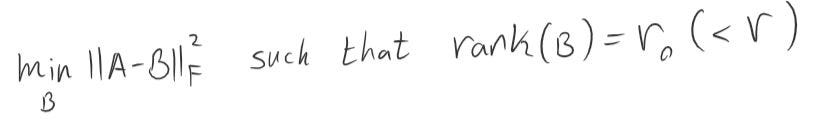
To solve this problem, we will need the following observation

Then, we can deduce that the solution to our problem is

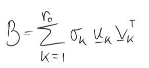
Simply put, the closest matrix B to matrix A is derived from the SVD decomposition of A. Assuming we want B to be of degree k, we will take the first k singular values, first k columns of U and first k rows of Vᵀ and get the closest we can get to A with degree k.

The moment has finally come, we get to see how does it work on a real image.

The code I wrote for this algorithm is right there if you wish to experiment with it on your own

For comparison, the image I compressed is the one in the top on a gray scale