Welcome back! In my last article Formal Truth and Logic we introduced many fundamental concepts (e.g. “What precisely is a ‘statement’?” or “How can we compose logic statements?”) of logic in Mathematics. If you require extra context on the notations or definitions used throughout this article, I highly recommend reading the previous article in case you have not done it already.

Mathematics as a science is in a distinguished position compared to most other sciences. This is due to its ability of making statements which are universally true (or false) based solely on the initially laid out assumptions of a statement. Why is that significant? It allows to draw conclusions deductively — meaning that conclusions preserve the truth of their original statements (s. [1] p. 5).

It is converse to induction, the way that empirical sciences advance: Inductionbuilds on collected evidence to generalize from individual observations to a general principle. Scientific methods nowadays are highly sophisticated. They are intended to minimize the likelihood of drawing flawed conclusions from well-designed studies. But the defining factor in this process is human judgement and the rigorous application of these methods in good faith. After all this, the result is still an approximation whose initial assumption of uniformity —that the studied phenomena can reasonably be extrapolated from the past into the future — has not and in most instances cannot be validated (s. [1] ibid.).

If we build on the other hand on statements that are known to be true to construct new statements which preserve this trueness, then we can substitute these statements as new primitives for further deductions. They follow the pattern “If X is true, then Y” or “Given X, then Y”. This way we gradually build up a tree of knowledge, in which every node is a universally valid statement only qualified through its specified premises and no other undefined environmental factors. Its validity is given by the strict application of deductive rules and the prior more primitive statements which allow to relate assumptions to the conclusion, tracing back all the way down to the fundamental axioms.

Proofs to Begin With

It all starts with a statement. The statement alone could possibly be true, possibly not. This statement is called a conjecture and becomes a theorem, once it has successfully been proven true.

Theorem: For two positive numbers a, b ∈ ℝ, if a < b then 0 < b -a.

Proof: The order axioms apply to the set of real numbers ℝ. This includes the law of monotony, which states that if a < b, then also a + c < b + c. That means a < b ⇔ a + (-a) < b + (-a) ⇔ 0 < b-a, the initial statement (s. [5] p. 293f).

Proofs and theorems build on each other and create a hierarchy. In textbooks this hierarchy is often directional from the more fundamemtal to the more advanced topics as the theory is gradually built up. Theorems and proofs are introduced in a didactically sensible order to support the later more complex concepts.

Theorem: For two positive numbers a, b ∈ ℝ if a < b then -b < -a.

Proof: The previous theorem states that a < b implies 0 < b-a. Hence, a < b ⇒ 0 < b-a ⇔ 0 < -(-b)-a ⇔ 0 + (-b) < -(-b)-a + (-b) ⇔ -b < -a (s. [5] ibid.).

But you could well imagine that there are many valid ways that lead to success. A more advanced property or concept could lead to a more elegant more concise way to derive one and the same theorem.

A proof does not necessarily need to adhere to a formal structure. Its logical structure and conclusiveness alone must be evident. A proof can hence be surprisingly sparse in words:

Theorem: Let c denote the length of the hypothenuse and a and b denote the lengths of the other two sides of a right-angled triangle, then a² + b² = c².

Proof:

Theorems and Lemmata

More often than not, the complexity of the relationship between different objects and their properties requires a strategic approach. The properties on which the to-be-proven theorem leans itself though can be extremely specific in their scientific merit to the surveyed relationship. In other words: Sometimes, premises required to prove your theorem are just way too specific to what you are currently trying to do.

Similar to how in good software engineering one decouples the interface of a function from its implementation, mathematicians often preceed their main theorem with a series of one or more lemmata. Structurally, a lemma is a supportive theorem: A proven statment describing a relationship between a number of premises and a conclusion. They serve to derive those aformentioned highly technical properties, which in turn make it possible to cleanly and concisely prove the main theorem. Or, they split the underlying components of a theorem into separate components— Divide-And-Conquer style.

The Root of All Proofs

So, proofs build on one another. But what lies at the root of them? As children we might have been asked this as a brain teaser: Define a term, an object, or a concept, without using this term or any of its synonyms in its definition. In Mathematics, we would like to have a logically constructed system, too, without self-references or any of its definitions relying circularly on one another.

This is where axioms come in: Elementary statements defined to be true (s. [5] p. 287). How is that possible? Well, defining something to be universally true without providing proof is only possible via general consensus. Yet, the set of fundamental axioms is carefully chosen to support the entire existing body of knowledge. There are several — admittedly informal — quality criteria for an axiomatic system to be recognised as such:

• Each axiom should be logically independent, i.e. it should not be decomposable into separate more elementary statments, not even into other axioms.
• The system should be conistent, i.e. under no circumstance should it be possible to derive a contradiction under that system. A contradiction occurs if for two statements A and B we can legally derive both A → B and A → ¬B under the same logic system. Such a system would be considered inconsistent.
• Ideally, we would like such a system to be also complete, i.e. we would like every true statement to be derivable under that system. However, this criterium is a weak criterium, as it has been proven that a system that is consistent, cannot be fully complete at the same time.

Could we prove an axiom wrong? And if we did, would that bring down all of modern Maths? Frankly, nothing would stop us from trying. But it would propably not lead to the fall of Mathematics as we know it. The reason for that lies in the selection process of the axioms: They are selected to match and describe intuitive properties of Mathematical objects like sets, fields, and numbers, that we can observe as we follow a Mathematical thought chain.

A good example are the order axioms which describe the ordering properties of all number sets from the natural numbers ℕ to the real numbers ℝ (cf. [5] p. 289). Showing that one of its axioms violates the consistency criterium, does not disprove the ordering property over ℝ per se, but it proves that our description of this fundamental property was inconsistent. If you can define a set on the other hand, which violates these axioms by design, then the ordering property simply does not apply in this set, meaning any other theorems derived from the order axioms would not apply either.

One other example comes from the field axioms, which state that a mathematical field 𝔽 satisfies these properties (cf. [4] p. 50f; s. [5] p. 288):

1. Addition over 𝔽…

• … is commutative.
• … is associative.
• … contains a neutral element 0 ∈ 𝔽 such that 0 + a = a for any a ∈ 𝔽.
• … has for every a ∈ 𝔽 an inverse element -a such that (-a) + a = 0.

2. Multiplication over 𝔽…

• … is commutative.
• … is associative.
• … contains a neutral element 1∈ 𝔽 such that 1 ∙ a = a for any a ∈ 𝔽∖{0}.
• … has for every a ∈ 𝔽∖{0} an inverse element a⁻¹ such that a⁻¹ ∙ a = 1.

3. Addition and Mulitplication over 𝔽…

• … is left-distributive.
• … is right-distributive.

It should be fairly easy to spot that all these properties apply to the real numbers ℝ and the rational numbers ℚ. But does it apply to the integers ℤ? Intuitively, we might guess, yes: Addition and multiplication are both commutative, associative and distributive over ℤ. We can name the neutral elements of addition and multiplication: 0 and 1.

What about the inverse elements? The additive inverse element for any integer ais -a. The multiplicative inverse element for any integer a is a⁻¹. In the case a = 1 or a = -1 the inverse element is a⁻¹ = 1⁻¹ = 1. If a = 2, the inverse element is 2⁻¹ = ½, which is obviously not an integer (s. [4] p. 48). By virtue of our defined axioms, we can conclude that the integers ℤ do not fulfill the qualities of a mathematical field (cf. [4] p. 51 and p. 63f).

Strategies for Proving

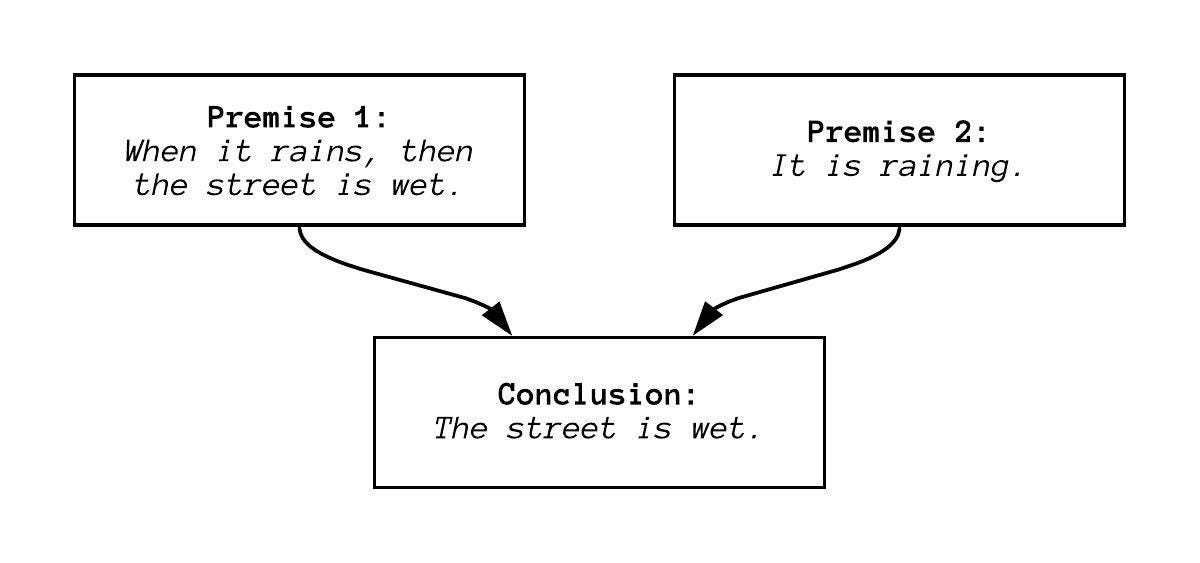
In Maths, theorems are used to state facts about the relationship between multiple statements. They are of the form

(1) A₁ ∧ A₂ ∧ … ∧ Aₙ → B

where the statement B is called the conclusion and the statments

(2) A₁ ∧ A₂ ∧ … ∧ Aₙ = ⋀︁ᵢ₌₁ⁿ Aᵢ

are called the premises. This type of statement is called an argument and it is considered a valid argument if when all premises Aᵢ are true, the conclusion B is true as well (s. [6] p. 597). In other words: For the argument to be valid, the conclusion can be never be false if all the premises are true. This matches our definition of an implication from our last article, the Introduction into Mathematical Logic. Remember, that we defined an implication itself to be false if and only if we attempt to imply something false from a correct statement.

A theorem is accompanied by a proof, deducing the conclusion from the inital premises. One little subtlety to consider: Desigining our argument such that it qualifies as valid is a premise in itself. What we are interested in is whether we can legitimately conclude statement B from the implication. Thus, suppose ⋀︁ᵢ₌₁ⁿ Aᵢ = A, then the logic structure of a proof takes the form

(3) (A → B) ∧ A → B.

Direct Proof

A direct proof is the simplest form of a proof matching the structure of statement (3). Setting the premises A as given, we derive conclusion B by sequentially applying axioms, definitions, and other theorems (cf. [4] p. 31).

The initial examples further above in this article all are examples for direct proofs.

Proof by Contradiction

Often times, it could prove difficult to show that A → B is true, as opposed to showing that the opposite ¬(A → B) is false. If ¬(A → B) leads to a contradiction, it must follow that A → B is correct (s. [4] p. 31f; [6] p. 618). The statements A → B and ¬(A∧¬B) are equivalent — I encourage you to verify this yourself by comparing their truth tables. Thus, if we would like to prove a statement of the form “If A, then B…”, we could instead phrase it as “Suppose A and ¬B…” and try to reach a contradiction (s. [3] p. 102f).

The probably most prominent application of proof by contradiction is the proof that shows that the square root of 2 is irrational:

Theorem: √2 is an irrational number (i.e. it cannot be represented as a fraction with both an integer numerator and an integer denominator).

Proof: Suppose for a moment that √2 were a rational number, then it would be possible to represent √2 as a simplified fraction with a, b ∈ ℤ:

(4) √2 = a / b ⇔ 2 = a² / b² ⇔ a² = 2b².

2b² is definitely an even number, therefore a² must be even. Suppose a were an odd number. That means, you could write a as 2k + 1. Inserting into a² yields:

(5) a² = (2k + 1)² = 4k² + 4k + 1.

But this is contradicting our statement, that a² must be even. Hence, a must be an even number, too. We can write a as 2k and insert again into a²:

(6) a² = 2b² ⇔ 4k² = 2b² ⇔ 2k² = b².

Thus, also b must be an even number. Since a and b must evidently both be even numbers, this contradicts our initial statement, that a / b was a simplified fraction. Ergo, it is not possible to represent √2 as a rational fraction and √2 must be irrational (s. [5] p. 319).

Proof by Contraposition

Although — as stated before — , the statements A → B and B → A are emphatically not equivalent, the statements A → B and ¬B → ¬A on the other hand, very much are (cf. [3] p. 51 and 96f; s. [4] p. 31). This becomes evident when comparing their truth tables:

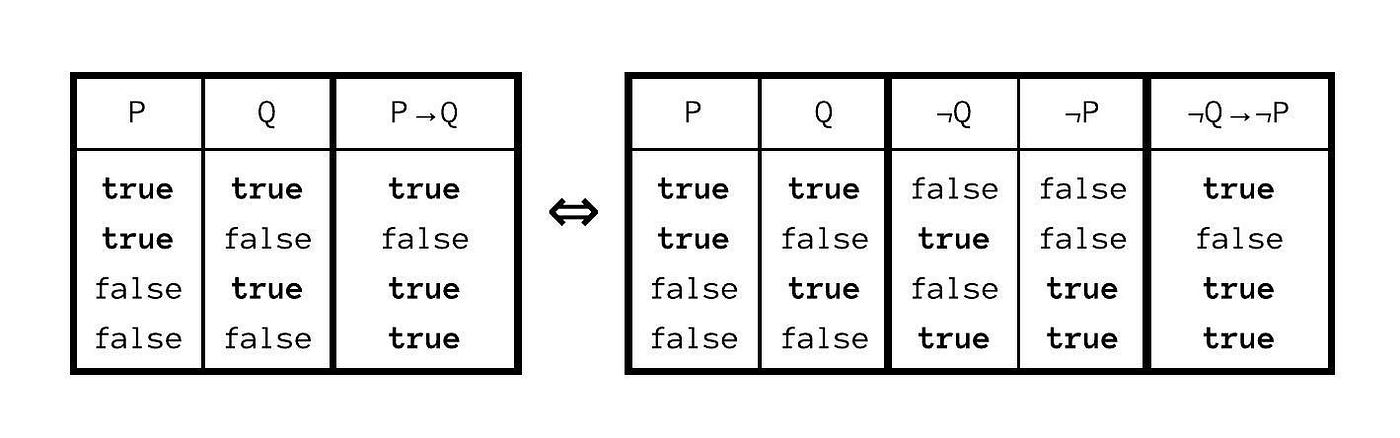
So, similar to proof by contradiction, if it appears difficult to show that A → B, it might instead be easier to show ¬B → ¬A, which is called proof by contraposition. More intuitively, the statements

(7) “If I called my mother, then she would be happy.”

and

(8) “If my mother is not happy, then I did not call her.”

convey the same relationship between the two statements “I called my mother” and “My mother is happy”. On the other hand, it would be impossible to extrapolate the same information from the statement

(9) “If my mother is happy, then I called her.”

Given statement (7) there is not enough information to determine whether statement (9) is equally true.

Theorem: For any a∈ ℝ, if a² is an even number, than a is also an even number.

Proof: We prove this theorem by contraposition, showing that if a is not even, that a²cannot be even either. Hence, suppose a is an odd number. It follows that a can be represented as an even number plus one:

(10) a = 2k + 1.

Squaring both sides gives

(11) a² = (2k + 1)² = 4k² + 4k + 1, which is always an odd number.

We have shown that if a is odd, then a² is necessarily odd, too. It follows that if a² is an even number, then a must also be an even number.

Proof by Mathematical Induction

Mathematical induction is working the same way we described induction further above, generalizing from an initial clause to a universal statement. Though, in this instance the induction is performed via strict application of deductive rules.

The significance mathematical induction has for Computer Science would easily warrant its own aritcle. It is particularly useful for statements that involve a form of discrete repetition, like sequences, series, summation, etc. — generally any time we hear a sentence like “Show that for all n ∈ ℕ…”.

It begins with the induction hypothesis, the statement that we would like to prove. The first objective is to prove that the hypothesis is definitively true for one specific instance of n — the base case— for example n = 1. In the next step we assume the hypothesis to be true, for arbitrary n ∈ ℕ. We try to show that if we take as given that the hypothesis applies to any n (and we already know one specific n, for which we have proven it to be true), that this implies the hypothesis to apply to n + 1 without any further restrictions. This is called the induction step (s. [4] p. 27).

So, suppose P(n) with n∈ ℕ to be the above mentioned induction hypothesis, we first show that P(1) is true. Then, assuming that P(n) were already proven, we show that P(n + 1) must equally be true. If we succeed, we can start again with the one case that we have already proven P(n = 1) and deduce that P(n = 2) must evidently be true as well. Given that P(n = 2) has now also been proven, P(n = 3)must also be true and so forth, proving P(n) automatically for all n∈ ℕ.

Theorem: Let n, m ∈ ℕ with n ≤ m and let A be a set with m elements. There are ∏ᵢ₌₀ⁿ⁻¹(m-i) ways to choose n elements from A, where each element in A can be chosen only once.

Proof: Let P(n) be the statement, that ∏ᵢ₌₀ⁿ⁻¹(m-i) is the formula for calculating the number for ways to choose n elements from a set A of size m. We prove P(n) via induction over n.

Base case: Let n = 1. There are m ways to choose exactly 1 element from A:

(12) ∏ᵢ₌₀¹⁻¹(m–i) = (m–0) = m, so P(1) is true.

Induction step: Assuming P(n) holds for any n, then P(n+1) must also hold true. We have to show that there are ∏ᵢ₌₀ⁿ⁺¹⁻¹(m-i) ways to choose n+1 elements from A. For every (n+1)ᵗʰ element that we choose, there are n elements that have already been selected and removed from the available choices. It follows there are (m-n) elements left from which to choose. The rule of product says we can multiply the number of choices for the (n+1)ᵗʰ element with the number of ways to choose all the previous n elements. Therefore, the possible number of ways to choose the first n+1 elements is:

(13) (m-n) ∙ ∏ᵢ₌₀ⁿ⁻¹(m-i) = ∏ᵢ₌₀ⁿ(m-i).

The statement P(n+1) evidently holds true, establishing the inductive step. Since the base case and the inductive step have both been shown to hold true, it follows that the initial statement P(n) holds for every n ∈ ℕ.

Proving the Equivalence of Two or More Statments

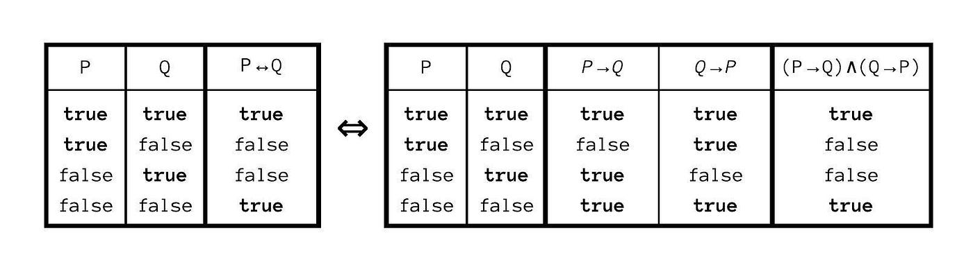
Bear in mind, that we had stressed in the last article that an implication alone is unidirectional. That means, that the statments A → B and B → A have strictly different meanings. To show the equivalence A ↔ B of two statements A and B, it is necessary to show that the implications A → B and B → A are each true individually (s. [3] p. 53f; [4] p. 31).

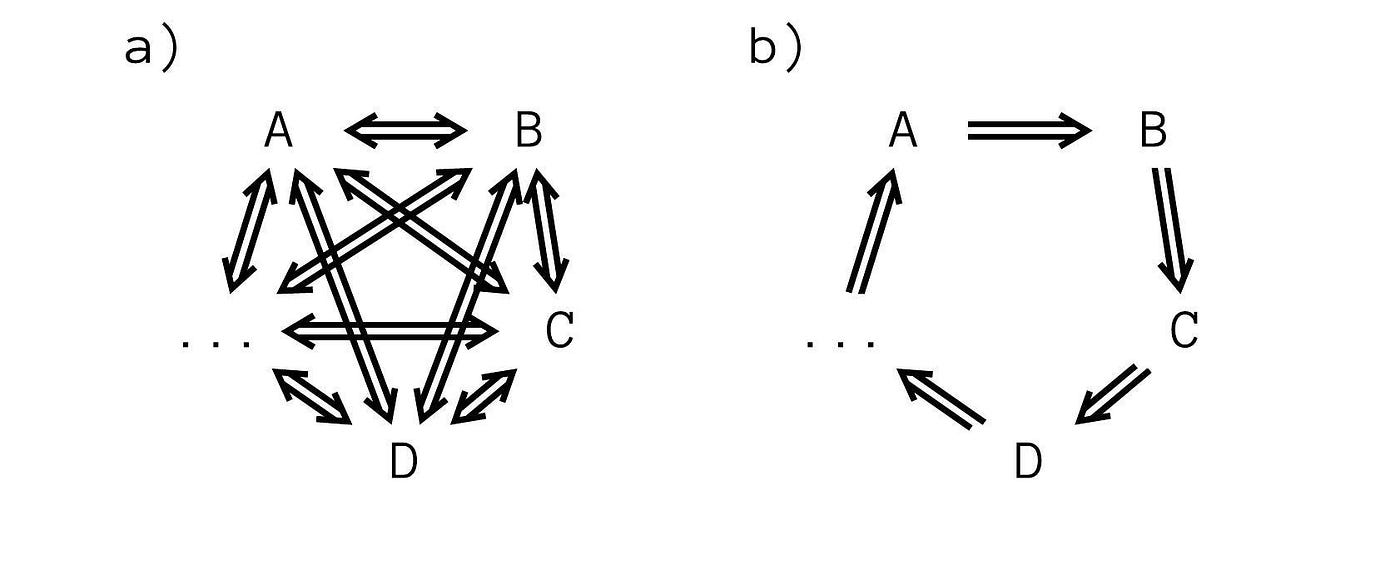
With 3, 4, 5 or even more statements that are all supposedly equivalent the number of pairwise implications to prove grows very rapidly (s. Fig. 5.a).

But implications are transitive, meaning that if A → B is true, and B → C is true, it follows that A → C is also true. And if A → B, B → C and C → A are all true statements, then by their transitive property we have already provided sufficient proof that A ↔ B ↔ C, i.e. that all three statements are in fact equivalent — again, I encourage you to compare their truth tables and verify this yourself.

So, to show that the statements A, B, C, … all are equivalent, we can line them up in an implication chain A → B, and B → C, and C → …, and …→ A. If we can show that each statment in the line correctly implies the next, then we have established the equivalence of all the statements in the chain (s. [4] p. 32). Note that the very last statement in the line must be shown to imply the first statement as well, to form a closed and valid implication circle (s. Fig 5.b).

Conclusion

We would like to think of proofs — just as we would probably like to think of any scientific statement — as giving us insight into a deeper causal relationship. But, if we were to relate two seemingly unrelated phenomena together and could prove that this relationship is true for all possible evaluations of the argument, then what does this tell us about its validity? What precisely does it tell us about its causality? The logicists view has been that Mathematic statements derive their truthness “by virtue of their form” (s. [2] p. 208), meaning the correctness of their syntactic structure and the mechanical application of inference rules, but distinct from their semantic meaning. Consequently, logic as a discipline strictly distinguishes between the syntax and the semantics of logic expressions (cf. [6] p. 582ff).

Although this article concludes our introduction into foundational logic in Mathematics, it would be interesting to pick apart what precisely this last bit means. I might pick the topic up one more time in a future article, delving deeper into statement and predicate logic. The direction forward though, will be to move to topics where what we have learned about logic arithmetics and proofs will become very relevant in an applied setting.

For example: what we have learned serves excellently as a bridge to digital logic, paving the way to talk about the architecture of computer systems. Hope to see you there!

References

[1] A. Schulz, L.Schlipf, and J. Rollin: Einführung in die wissenschaftliche Methodik der Informatik: Wissenschaftstheorie. Kurseinheit 2, Volume 2, FernUniversität, Hagen, 2019.

[2] E. Snapper: The three crises in mathematics: Logicism, intuitionism and formalism. Mathematics Magazine, 52(4), 1979, p. 207–216.

[3] D. J. Velleman: How to Prove It: A Structured Approach. 3rd ed., Cambridge University Press, Cambridge, 2019.

[4] L. Unger: Mathematische Grundlagen: Grundlagen. Kurseinheit 1, Volume 1, FernUniversität, Hagen, 2019.

[5] L. Unger: Mathematische Grundlagen: Reelle Zahlen und Folgen. Kurseinheit 4, Volume 4, FernUniversität, Hagen, 2019.

[6] L. Unger: Mathematische Grundlagen: Etwas Integralrechnung und viel Logik. Kursheinheit 7, Volume 7, FernUniversität, Hagen, 2019.