Throw back (or forward) to your high school math classes. Remember that one lesson in algebra about the graphs of functions? Well, try visualizing what a parabola looks like, perhaps the equation y = x². Now, I know what you’re thinking: How does this simple graph relate to this article’s title? To how machines learn? Well, it actually points to one of the fundamental concepts of machine learning — optimization.

What is a Loss Function?

In typical machine learning problems, there is always an input and a desired output. However, the machine doesn’t really know that. Instead, the machine uses some of the input that it is given, as well as some of the outputs which are already known to use in predictions. Determining the best machine learning model for a certain situation often entails comparing the machine’s predictions and the actual results to determine whether or not the algorithm used is accurate enough. The problem is, how do we know whether or not the machine is learning effectively? This is where optimization enters the picture in the form of a loss function.

To increase accuracy, the value of the loss function must be at the minimum. An example of a simple loss function is the mean-squared-error (MSE) which is given by the expression below:

Here, n refers to the number of data points; yi, the actual output; xi, the machine’s prediction.

From this, we can see that the MSE evaluates (yi-xi) for every data point in the input. Each iteration and evaluation of the loss function for each data point is called an epoch. In a working machine learning model, the loss function decreases with the more epochs it iterates through.

We can optimize a model by minimizing the loss function. Intuitively, we can think of the loss function as the accumulation of the differences between the prediction and actual value for each data point in a certain dataset. Hence, maximum accuracy is achieved through minimizing these discrepancies.

Defining Gradient Descent

Now, let’s examine how we can use gradient descent to optimize a machine learning model. Of course, we have to establish what gradient descent even means. Well, as the name implies, gradient descent refers to the steepest rate of descent down a gradient or slope to minimize the value of the loss function as the machine learning model iterates through more and more epochs.

In this model, we can see that as the number of epochs increases, the machine is able to better predict the output of a certain data point. The value of the loss decreases, and by the 10th epoch it’s already pretty close to 0 which is what we want.

Our Parabola and Tangent Lines

Now, let’s go back to our parabola (hopefully you’ve kept this in mind). How do you think gradient descent can be applied here? Ideally, we would want lines to obtain gradients, but it doesn’t seem too obvious especially since our parabola is curved. At first, it may not seem too obvious, but there’s actually a way to conquer this minor obstacle. Given that our goal is to achieve the minimum, this begs the question: “At what point on the graph do you think the minimum value of the loss function (which models a quadratic equation) lands?” It would be at the vertex (A), of course!

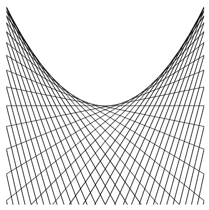
You might be asking yourself, “How can this simple graph be related to gradient descent?” The lines we’re looking for aren’t formed by the graph itself, but instead, they’re actually the tangent lines for each point on the graph. Tangent lines are lines that intersect the graph at only one point and can reveal how gradient descent works. To appreciate the beauty of such lines, let us marvel at the aesthetics of this visualization:

Going back, for simplicity, let’s draw a tangent line for a random point B. Then, we also draw the tangent line for our minimum point (vertex) as shown:

Of course, the objective is for B to eventually approach or even reach A. Here, the slope of the orange tangent is negative and non-zero. This tells us two things: the “direction” in which B should go and that the magnitude of the slope should decrease towards 0. “Why 0?”, you might ask. Since A is the vertex of the parabola, its tangent line would be a horizontal one. We can then calculate its slope as follows:

In the context of a machine learning model, iterations through each epoch should ideally bring B closer and closer to A. However, the number of epochs that need to be run through affects how quickly this is achieved. The number of epochs needed is in turn affected by a “learning rate.” You can think of the learning rate as the “step-size” that B traverses down the graph. We can then take the gradients for every point that B lands on until it eventually reaches 0 (which is precisely at A).

Adjusting the Learning Rate

However, there is a caveat for the learning rate. If the learning rate or “step-size” is too high, there is a possibility that B may never reach or become close to A, thereby decreasing the model’s accuracy. In short, it may overshoot or diverge from the minimum.

Here, following the blue lines simulating the path of B, it may originally seem that the model is doing relatively well as B approaches closer to A. However, B eventually diverges from A, as shown by the purple line, due to overshooting.

On the other hand, if the learning rate is too small, B may take more epochs than necessary to approach A and approach it very slowly.

Here, following the blue lines which simulate the path of B, we can see that B takes very small “steps” per epoch. Although this model would be accurate, it would not be too efficient.

Epilogue

In this article, we discussed gradient descent through the visualization of a quadratic equation (a polynomial of degree 2). However, in reality, large-scale machine learning problems often involve hundreds of different types of inputs (also called features) which increase the degree of the polynomial for the loss function. Despite this, the end goal remains the same: minimize the loss function to maximize accuracy.

I am in no way, shape, or form, a machine learning expert. However, as a cornerstone of machine learning, gradient descent is simply something that I believe everyone should be familiar with. That being said, I hope that this brief explanation helps in introducing you to the ML world. Thanks for reading!