In 1983, Gerd Faltings proved a long-standing conjecture of Mordell from 1922. The statement and proof of this theorem illustrate just how connected many disparate branches of math are.

I won’t state it in its original form, but there is an easily understandable modification of it that will probably come as a surprise to many readers.

This article will try to give some idea of the statement and proof, but mostly, I hope people come away awed by how number theory (study of prime numbers and integers) can be connected to geometry, complex analysis (study of calculus with imaginary numbers), and even topology (study of how shapes stretch and deform).

Zeroes of Homogeneous Polynomials

To start with, we’re going to think about homogenous polynomials in three variables with rational number coefficients.

A homogeneous polynomial is just a polynomial where each piece has the same degree.

Some examples are x²+(1/2)y²-z² and x³+xyz + yz². The first one is degree 2 because all exponents are 2. The second one is degree 3, because if you add the exponents on that middle piece it’s 1+1+1 and on the last piece it’s 0+1+2.

Hopefully, that makes sense.

Examples that we will not consider are things like x²+y+xz³+1. This has different degrees on each piece, so it’s not homogeneous. We also won’t consider πx³-π²y³. This is homogeneous, but it doesn’t have rational number coefficients.

Notationally, our homogeneous polynomials are elements of the ring ℚ[x,y,z]. You can ignore that if you haven’t seen it, but I will default to using this notation when convenient.

We’re going to consider rational solutions when we set the polynomial equal to 0.

If p(x,y,z) is a polynomial, then a rational solution is a triple (a,b,c) of rational numbers such that p(a,b,c)=0.

For example, the degree two homogeneous polynomial x²-z² has the rational solution (1,0,1) since 1²-1²=0. It also has the solution (1,1,1) and infinitely many others.

Here are two facts about homogeneous polynomials.

Fact 1: If the degree is at least 1, then (0,0,0) is always a solution. Convince yourself of this.

Fact 2: If (a,b,c) is a rational solution, then we can multiply that solution by any rational number and get another rational solution. In fact, finding rational solutions is basically equivalent to finding integer solutions, because we can multiply by the denominators of a, b, and c in order to get a whole number solution.

This second fact is just factoring. Again, this is an exercise for you if you’re not convinced.

Hint: Let (a,b,c) be a solution. If the degree of p(x,y,z) is d, then:

p(λa, λb, λc)=λᵈp(a,b,c)=0.

When we get to the geometry later, this second fact is our motivation to work in projective space. We won’t worry too much about that, but the exact definition of projective space is to throw out (0,0,0) and then consider multiples of (a,b,c) to be the “same.”

We’ll call two solutions distinct if they aren’t multiples of each other.

Low Degree Examples

Let’s take some time to think about how many distinct rational solutions there are in some low degree examples.

Degree 1 is easy and completely solvable. There are always infinitely many distinct rational (and hence integer) solutions, and you can see this using a “trick” that turns out to be useful in the degree 2 case.

You can plug in 1 for one of the variables and you’ll be left with 2 variables. Then solve for one in terms of the other and start plugging in.

If p(x,y,z)=x-y-z. Then plug in z=1 and set it equal to zero and solve. You end up with x=y+1. This is essentially “parametrizing” an infinite collection of solutions.

For any rational number a, we get that (a+1, a, 1) is a distinct solution.

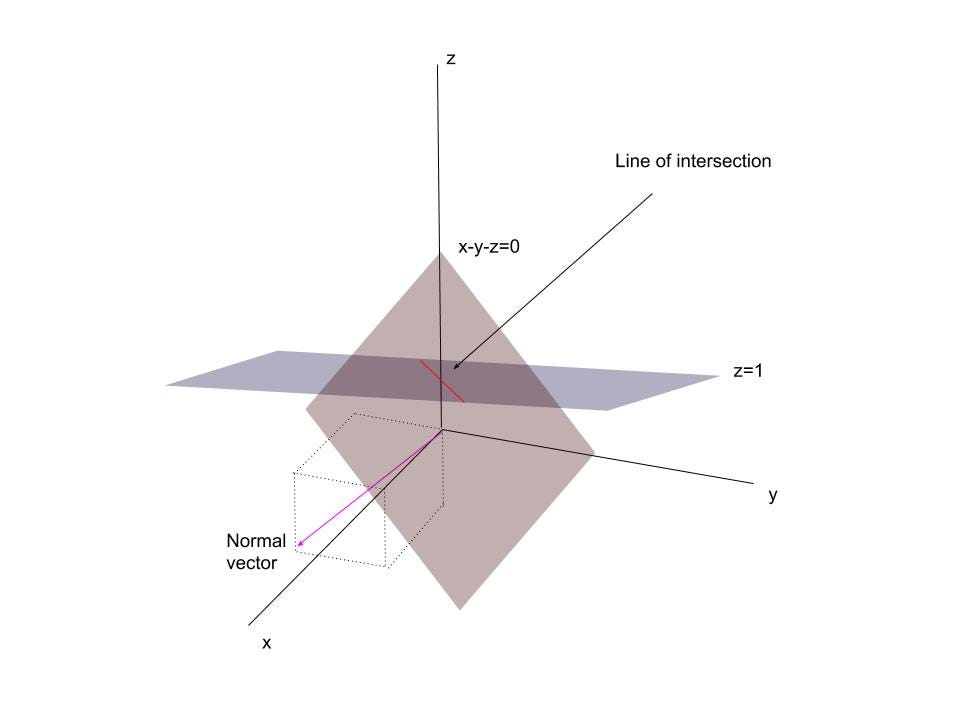
Geometrically, you might know from linear algebra or calculus that x-y-z=0 is a plane with normal vector <1,-1,-1>. By setting z=1, we are intersecting it with another plane (the xy-axis shifted up by 1 unit).

The intersection is the line we parametrized.

You might think this was weird. Why did we set z=1? But we’re basically trying to answer the question: are there infinitely many distinct rational solutions? This trick didn’t give us all solutions; it just gave us an easy way to test whether there were infinitely many.

For degree two, things get interesting. Let’s take a polynomial you know well: x²+y²-z². If we set this equal to 0, we x²+y²=z².

In high school, you probably learned that there were infinitely many “Pythagorean triples,” and so this also has infinitely many distinct rational solutions.

I don’t want to dwell on that too much. Proofs are abundant with a Google search, but they’re a bit too long a tangent for this article. Instead, let’s shift to the geometric picture again.

The graph of x²+y²=z² is a cone.

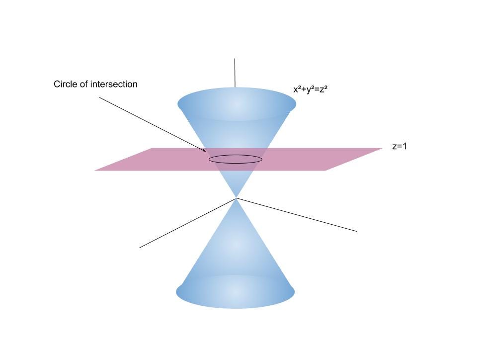
When we set z=1 again, we get x²+y²=1, the well-known “unit circle.” And the problem gets transformed into proving there are infinitely many rational points on the unit circle:

This is a well-known fact, but the proof is essentially the same as proving infinitely many Pythagorean triples. So we’ll skip that.

Here’s one more thing before we move on. There are degree 2 polynomials with no rational solutions (remember we’re throwing (0,0,0) out). For example, x²+y²+z².

But if we allow adjoining a single root of a polynomial to ℚ, then we get infinitely many solutions. For example, if we adjoin i (a root of x²+1), then we could set z=i. This converts the equation to x²+y²=1 again, and so we get infinitely many solutions over ℚ(i).

This is an amazing fact about the degree 2 case: there are either no solutions or infinitely many. In the case that there are none, you can always adjoin a single root of a polynomial to ℚ to get infinitely many.

The degree 3 case has the same property. There’s either no solution or infinitely many (and you can adjoin a single root of a polynomial to get infinitely many).

Proving this is much harder, but as a teaser, it has to do with the fact that over the complex numbers, degree 3 polynomials define elliptic curves.

Falting’s Theorem and Fermat’s Last Theorem

Now we can basically state a modified version of the Mordell conjecture that Faltings proved.

Let p(x,y,z)∈ℚ[x,y,z] be a homogeneous polynomial. Suppose also that p(x,y,z)=0 is “smooth.”

Please don’t get hung up on this condition. It has to do with the fact that the theorem is fundamentally geometric, not algebraic. I’m giving you an altered version. The smooth condition can easily be checked using usual calculus methods (taking partial derivatives).

Theorem: If the degree of p(x,y,z) is greater than 3, then there are only finitely many distinct rational solutions. Moreover, you can never obtain infinitely many solutions by adjoining finitely many roots of polynomials to ℚ.

The first thing to note is that this gives us a weak form of Fermat’s Last Theorem, since xⁿ+yⁿ=zⁿ is a special case of this. This is usually referred to as “Finite Fermat,” since it says that for n≥4, xⁿ+yⁿ=zⁿ only has finitely many integer solutions.

I’ll just throw in that the theorem tells us when there are only finitely many solutions to some non-homogeneous polynomials by plugging in z=1 as we did in the examples above.

It’s possible to homogenize a two-variable polynomial to a three-variable homogeneous one, but you often introduce non-smooth points. So I don’t want to get into the subtleties of that.

The theorem is definitely not true if you drop the smooth condition.

I’m going to keep with the homogeneous version, but you might see this other statement in some places.

Some Topology

We’ve been doing something that probably seems normal to you, but it’s a little weird when you think about it.

We want to find integer solutions to a polynomial. In the examples above, we did this by thinking about geometry over the real numbers and then tried to go backward.

I did this on purpose to get you thinking in those terms. When we switch to think of shapes in ℝ³, we were able to rely on tools we knew from other subjects, like Calculus or Linear Algebra.

This concept of starting with something over ℚ and then switching to something over ℝ or ℂ, utilizing geometry or topology, and then going back at the end is one of the fundamental insights in a branch of math called “arithmetic geometry” (which was my research area).

The ℚ points of a geometric space are a subset of the ℝ points which are a subset of the ℂ points. Each time we add more to the space, we can think of this as filling it in with more and more.

We talked about this earlier, but instead of using ℝ³, we should actually use something called projective space. For reasons that shouldn’t be obvious right now, we should also work over the complex numbers (this basically makes it so we don’t “miss” any solutions like i).

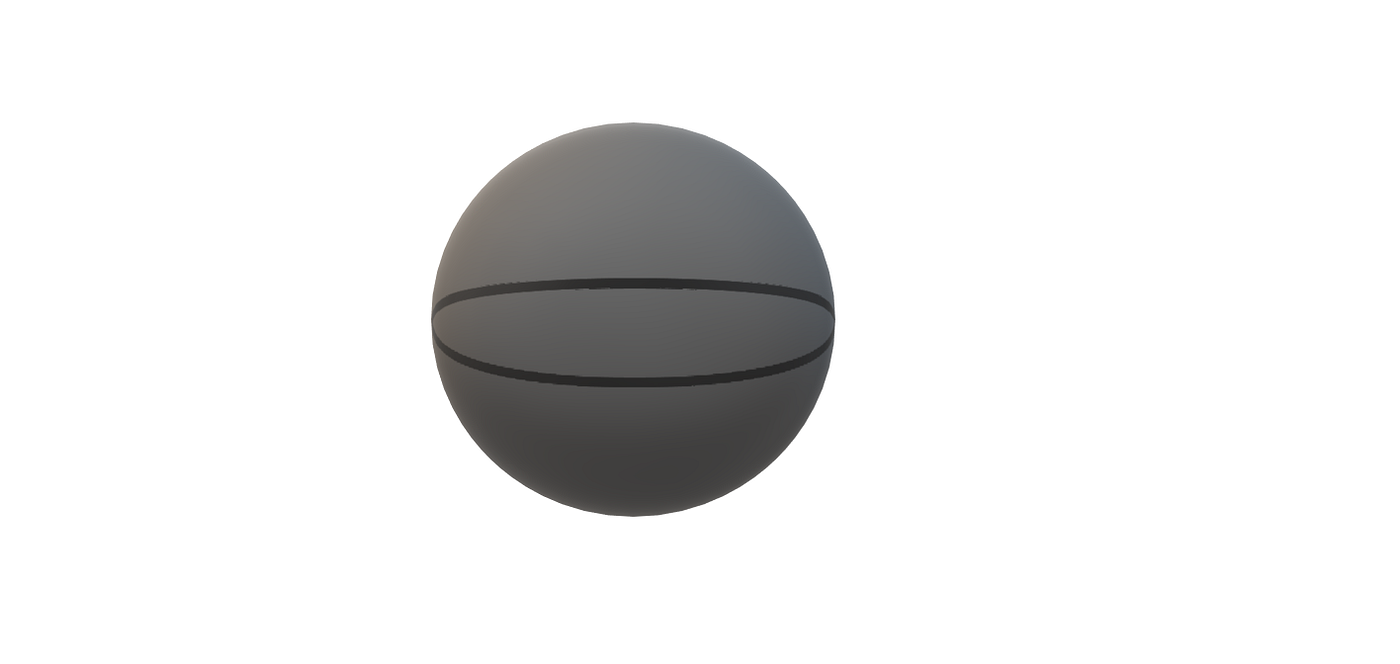
When we do this, our polynomial p(x,y,z) makes a really nice shape. When the degree is 2, it will always be a sphere topologically:

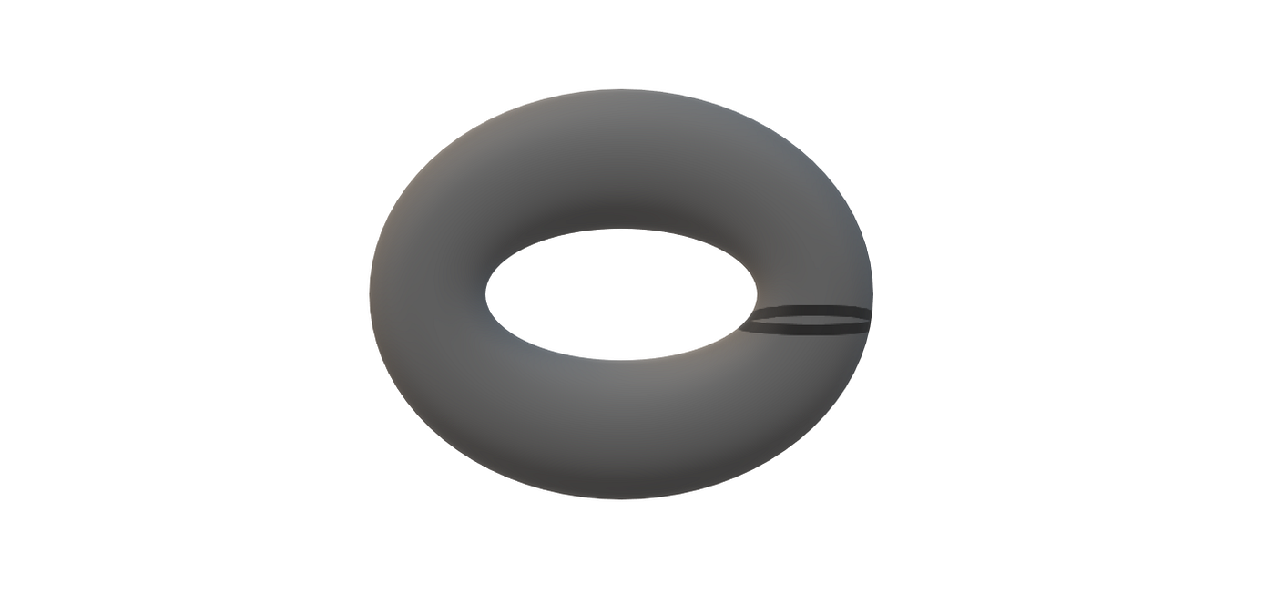
When the degree is 3, it will always be a donut topologically:

When the degree is 4, it will always be a shape with “3 holes” topologically:

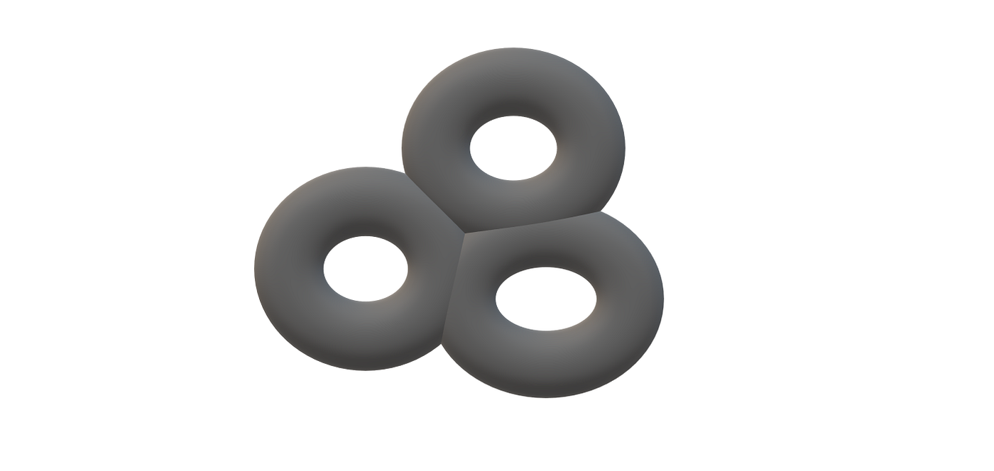
The number of holes is called the genus, g. The curve defined by a degree 2 polynomial has genus 0; a degree 3 curve has genus 1; a degree 4 curve has genus 3.

The connection between the degree of a curve and its genus is a really deep and subtle one. In general, it is given by the Genus-Degree Formula:

In case you’re concerned, these look like 2-dimensional objects (surfaces), but I’m using the name “curves,” which implies they are 1-dimensional.

This is just because the complex numbers look like ℝ². These geometric spaces have complex dimension 1 and real dimension 2. Don’t get caught up on this. Many people refer to these as “compact Riemann surfaces.”

You should notice something odd about the Genus-Degree Formula. There’s no way to produce a genus 2 shape. This is because we’re making curves out of a single equation — an extremely restrictive thing. These are usually called projective algebraic plane curves.

It’s a surprising fact to learn that there are no genus 2 plane curves. But, of course, there are genus 2 curves that can be produced in other ways.

This is why Faltings’s Theorem is usually stated as a fact about curves and not equations. It says that if you have any smooth projective curve of genus greater than 1 defined over ℚ, then there are only finitely many rational points on it.

The fact that topology is somehow coming into this should amaze you. We started by thinking about rational/integer solutions to an equation, and we’re finding out that it depends on the genus, a topological property.

De Franchis Theorem

Sketching the full proof of Faltings would be crazy to do in this article. It’s quite long and involves many brilliant insights.

But I do want to give a flavor of why genus comes up.

If you’ve taken a complex analysis course, then you might have seen why genus g≥2 is important.

Compact Riemann surfaces have three types (and they are pictured above).

Genus 0, spheres, are called elliptic. There are infinitely many ways to rotate it and keep it the same (isometries). In my article on modular forms, I talked about how to do this with linear fractional transformations PSL(2, ℤ).

Genus 1, donuts, are called parabolic. They are elliptic curves, and so it makes sense to add points to each other. Moving points around using this addition gives us infinitely many isometries again.

Genus bigger than 1 are called hyperbolic. They only have finitely many isometries, and this geometric fact is crucial in Faltings’s proof that there are only finitely many rational points for such curves.

One amazing thing to take away from this is that people who study differential geometry over the complex numbers already found this same distinction that g≥2 is special and gave these spaces a name: hyperbolic. This classification originally had to do with the curvature metric.

The main result we’ll need in the next section is the following. If X and Y are curves with genus bigger than 1 (possibly different), then the set of non-constant functions f: Y→X is finite. This is known as the de Franchis Theorem.

The fact that there are infinitely many isometries in the genus 0 and 1 case shows that this theorem is false in those cases.

Changing the Problem

Let’s reset now since I just threw a lot of stuff at you.

If we have a polynomial q(x,y,z), then the zero set forms a curve C. Since we’re going to make the curve in complex projective space, it might look a little different than you expect (it has 1 complex dimension or 2 real dimensions).

We can think of a rational solution (a,b,c) geometrically as a point, p, on the curve.

The main idea is to switch from the hard problem of solving a polynomial, to an easier geometric problem.

For each rational point, we’re going to construct a different object. Only finitely many distinct rational points will correspond to the same new object. This will change the problem to showing that there are only finitely many of this new object.

Hopefully, that made sense. It’s a really clever idea, so I’d recommend convincing yourself of it before moving on.

Every curve C has a g-dimensional space associated with it (where g is the genus of C) called the Jacobian variety, Jac(C). This new space is extremely nice: it has a way to add points. In fact, genus 1 curves are the same as their Jacobian (we already mentioned they have a way to add points earlier).

Given a rational point, p, on C, we can actually find a copy of the curve itself in Jac(C) with the property that p is the identity element (think of it as “0” when adding points).

It makes sense to “multiply by 2” on Jac(C) by just adding each point to itself. This produces a new curve of at least the same genus and a function f: D→C and moreover, the function is “bad” at p but nice everywhere else.

Here’s the idea in picture form (though it’s technically misleading since we’re forming a “pullback” if you know what that means):

So each rational point, p, on C gives us a new curve D (and a function f: D→C). This D has a different genus than C, but every D produced this way from distinct rational points has the same genus.

The de Franchis Theorem tells us that only finitely many distinct rational points on C can give us the same D or else we would have produced infinitely many f: D→C, a contradiction.

Let the genus of D be notated h. This transforms the problem to showing there are only finitely many curves of genus h. Technically, you need to keep track of some other information while doing this.

I should point out that this first reduction was originally proved by Kodaira and Parshin. So, this association of a rational point to a new curve is sometimes called the “Kodaira-Parshin construction” or “Kodaira-Parshin trick.”

This transformed problem is not easy, and in fact, the finiteness was conjectured by Shafarevich earlier. So this merely transformed the problem to something else unknown.

Faltings made several more reductions of this same type, where you only need to show finiteness of some other collection of objects, before completing the proof.

He proved this final collection actually was finite, and so the Mordell Conjecture is true!

In 1986, Faltings was awarded the Fields Medal (the highest award for mathematics), and it was largely due to proving this.