
Extending Einstein’s Field Equations
Wave Properties of Matter in Gravitational Fields

However much it has served, there is no clear consensus today on exactly where Newtonian gravitational acceleration originates, let alone what it is, except for what it does. In deed, the Oxford dictionary of physics defines gravity as “the attractive force by which bodies are drawn towards the centre of any celestial body, such as the Earth or the moon”. It is therefore described by its action — what it does, upon accepting the generic verb that of being an “attractive force”. The dictionary goes ahead to explain that its intensity is measured by the acceleration produced, and hence we cannot say in the most precise terms what it is, and where exactly it comes from.
In this essay, we will attempt to explain what it is, where it originates from, as well as present the mathematical evidences that supports the claims, and with minimal shake-up to the currently accepted scientific norms.
“… for every coordinate x,y,z,t used in Einstein’s description of gravitational field as the response variable, there is an extra frequency term, that exhibits wave-like properties”
Gravitational Fields
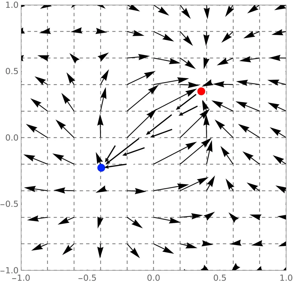
Einstein’s description of gravity, which is now widely accepted includes the fact that gravity is characterized as a field, meaning that it is a quantity in space that exists at each position bound by coordinates. Reference to fields is rare in our everyday conversations, as we prefer to simplify the quantities by lumping them up, and stating them over a larger extent. For example, we refer to quantities like temperature, by prefixing with the location in which the measurements were taken e.g. “room” or “wall” temperature. In the strictest terminology however, a field has different values at every tiny point (or coordinate) as depicted in Fig. 1 for a two dimensional field.

The labels are intentionally omitted in Fig. 1, to mean that they are positions in space, and can be in any type of selected coordinates. The most common coordinates are: number line, polar, cylindrical, homogeneous, and Cartesian coordinates. Einstein therefore used such a system to describe the presence of gravity in each x, y, z, and time coordinate — which he referred to as spacetime. Einstein’s work culminated to what we now know as Einstein’s Field Equations, which in the most simplified terms is usually presented in tensor form as follows:

Where Rₐ is Ricci’s tensor, R its trace, gₐ is the spacetime metric, Tₐ the matter energy–momentum tensor which includes the cosmological constant, G is Newton’s universal gravitational constant, while c takes the speed of light in a vacuum. Notice that Eq. (1) is referred to as field equations — in plural, to mean that it can further be broken down into many equations, ten of them to be precise. One of the methods of breaking down Eq. (1) is through Taylor series expansion — named after the British mathematician Brook Taylor who introduced the method in 1715.
Einstein’s field equations are generally known to be laborious and computationally intensive. As a matter of fact, Einstein himself did not believe that exact solution to his field equations would ever be obtained. He however went ahead in an attempt to solve them, albeit ending up with only approximate the solutions. The main source of errors in Einstein’s field equations is the aforementioned methodology, the Taylor series expansion which allows the error to propagate depending on the number of expansion terms used. It is therefore fair to say that his attempts were also limited by the finite computational resources available during his time¹.
Despite this difficulty however, there have been several attempts, with the first exact solution coming from Karl Schwarzschild a German physicist, astronomer, and a 1st world war veteran in 1915 — the same year Albert Einstein published the field equations. The solutions of Einstein’s field equations are referred to as metrics, and thus the Schwarzschild solution also goes by the name Schwarzschild metric. This solution in turn results in what is called Schwarzschild radius rₛ, and it describes the size of the event horizon of a non-rotating black hole. The mathematical formula is given as follows:

With time there have been other notable solutions to Einstein’s field equations, namely: Reissner–Nordström, Kerr, and Kerr-Newman metrics. All these methods also corresponds to the type of black hole they characterize. To summarize this section, the reference to gravity as a field still doesn’t answer the where from question. However, it rather tells us where it resides in our universe — in the field.
Gravity as a Curvature in Space
One other way of looking at gravity, is by considering it as a curvature in the spacetime matrix created by massive objects. This is a very common understanding of gravity, even though it does little to explicate not only the source of gravity itself, but can also be potentially misleading. Viewing gravity as a force that causes bending in spacetime confuses many readers as it does not explicitly describe for instance, what then causes the attraction as earlier observed by Isaac Newton — assuming two objects have different masses but sits on the same level ground.

In general, the understanding that comes from a combination of the two models is that, while we see Newtonian gravity as pulling force between masses at the same level “ground”, Einstein’s model quantifies gravity by the amount of “depression” effect or vortex created by the weight of the massive object in the spacetime matrix. Smaller masses therefore tend to try and occupy the vortex so created.
Spacetime-f: The Extension of Spacetime
The aim of this section is to show that for every coordinate x,y,z,t used in Einstein’s description of gravitational field as the response or dependent variable, there is an extra frequency term, that exhibits wave-like properties.
It is generally accepted that our universe is made up of pure frequencies. However, this thinking has not gone past the state of being a philosophical cliche, as far as mathematical logic is of concern, when it comes to objects of large extent. For example, there are exemplary methods to estimate the wave properties of elementary particles, amongst which are de Broglie and Compton wavelengths. Compton’s methodology was particularly revolutionary, as it allows us to determine precisely the rest mass of particles that would otherwise be incredibly difficult to measure. According to Compton scattering, the wavelength of a particle is equal to the wavelength of a photon whose energy is the same as its mass, and can be represented as follows:

Where h is the Planck’s constant, and c is the speed of light in a vacuum. There is one caveat however, when considering the use of Eq. (3) namely: It applies to single, homogeneous, particles and not composites. That means it may not apply to any particle of considerably large extent, let alone celestial bodies. For instance, if we were to calculate such a wavelength for planet Earth we would probably end up with trivial and less intuitive outcomes.
We would then be naturally compelled to find an equivalent of Compton formula for large objects that in everyday life would allow us to tag an object of whatever mass to a wave property, such as frequency or wavelength, and the answer comes from adding an exact solution to Einstein’s field equations. To get us started, for any object regardless of its dimensional extent, r and mass m, its Compton wavelength equivalent is given by the following formula:

Where rₛ is the Schwarzschild radius. The wave numbers for the above wavelength can also be obtained by simply taking the reciprocal κ=1/λ. A whole range of nearby planetary bodies has been presented in the Table 1 following the same methodology.

The first merit we get from transforming massive objects into their equivalent single-particle Compton wavelengths, is that their corresponding radio frequencies are obtained through the classical electromagnetic wave relation f=c/λ. Surprisingly enough, this opens up a new window of opportunity to estimate Newtonian gravitational potential, g as follows:

The simple explanation why this works for every celestial body be it a planet, the moons, neutron stars, and even black holes, is because the method can be reduced back to what we have always known to constitute Newtonian gravity. This can be done by carrying out the following steps:

Where M is the mass of the object in question. The second merit we get is that of characterizing celestial bodies from planets to black holes, including finding them. This can be done through any radio frequency mapping (radar) method upon which, the gravitational potential, g can then be obtained using Eq. (5), and the radii can be calculated with the following method:

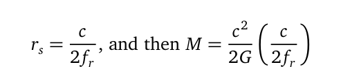
The minimum value r can take in Eq. (4) is rₛ, such that an object whose radius is less than or equal to its Schwarzschild radius is classified as a black hole. For such a system, Eq. (4) can further be simplified to λ = 2rₛ. The implication here being the properties of a black hole such as mass, energy density, and even Schwarzschild radius, can be estimated once the said radio frequencies have been obtained. For Schwarzschild black holes, the gravitational radii and the masses can then be estimated as follows:
We seem to know that stars such as our sun gradually losses their energy — referred to as nucleosynthetic power, albeit in infinitesimal amounts. The end expectation is the formation of a black hole at the centre. If we were to model such an event using this methodology, we would simply allow the wavelength to recede, say by an amount Δh=λ-r at any given instance. The metric solution form we end up with will then be expressed as follows:

This is to say that an object may not form a black hole as long as the difference Δh, between its radius and its corresponding wavelength is greater than rₛ. The only bottleneck in obtaining the wave frequencies relating to gravitational fields is a possible lack of accurate detection tools since these are ultra low frequencies (ULF) that lies in the extremes of the electromagnetic spectrum (see Fig. 3)
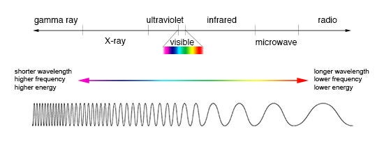
The frequencies we are searching for are found in the extreme right on Fig. 3. Meaning that they are long wavelength, and low energy in the orders of nano Hertz. For planet Earth, this value is at 32.71 nano Hertz. The highest being that of Jupiter at 77.05, and the lowest is Pluto with a frequency of 2.335 nano Hertz.
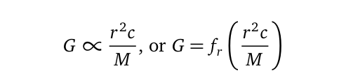
As a side note: The universal gravitational constant is not universal as it has always been thought of. It is rather a constant only relative to the planet in which calculations are done. That is to imply that the constant 6.6743E-11 only works for Earth. In the strictest definition it is a variable for each massive object as it is proportional to its extent r, mass M, and the proportionality constant is the surrounding frequencies discussed in this article.
The outgoing paragraph underpins the probable reasoning behind most attempts to apply general relativistic calculations to quantum mechanics totally goes sideways — in these cases G is in the orders of 10E-54 as discussed here.
Conclusion
There are compelling reasons to believe that every coordinate in a gravitational field described by Albert Einstein as spacetime can be associated with wave properties, that when leveraged enables further characterization of the field. In particular, massive objects in a gravitational field tend to cast a wavelength around them, that is much larger (in extent) compared to their own radii.
The wavelengths constitute radio frequencies that if properly mapped, can be useful in estimating a whole range of other properties relating to the gravitational fields upon which the objects reside. The methodology has therefore been dubbed spacetime-f as it adds a response frequency variable fᵣ, that is quantifiable for every single one of the coordinates x, y, z, and t positions. This therefore means mass is no longer the only way to detect curvatures in spacetime, but the sole notion of these radio frequencies are also good enough candidates for space exploration, provided they are within our electromagnetic spectrum.
A successful understanding and further implementation of these methods could also open up other technological pathways such as advances in sound navigation and detection ranging (sonar, sodar and radar) in microscales, not to mention the possibilities for anti-gravitation.
References
¹ Miller, Mark. “Accuracy requirements for the calculation of gravitational waveforms from coalescing compact binaries in numerical relativity.” Physical Review D 71.10 (2005): 104016.
² https://science.nasa.gov/science-news/science-at-nasa/2005/16nov_gpb


