Analysis

Distributions: What Exactly is the Dirac Delta “Function”?

The theory of distributions , also known as generalized functions, often remains something of an enigma…

Adam Taylor

Sep 20, 2020 — 15 min read

The theory of distributions, also known as generalized functions, often remains something of an enigma to practicing physicists and engineers, even those working on heavily mathematical projects. This is especially true for the author, who despite the efforts of very capable instructors in graduate courses on distributions, Sobolev spaces, and the like, managed to get through without really internalizing the key points. The present article represents the fruits of my attempt, years later, to remedy the effects of my own laziness and stupidity. It is my hope that it may help to provide some clarity to those who may be in the same position. To blatantly steal from an old and famous calculus text [1], “what one fool can do, another can.”

It is my personal belief that mathematical concepts, no matter how abstract, are most easily digested when given some historical contextualization. Ideas can seem totally foreign when abstracted from the environments in which human actors invented them for specific purposes. Often mathematics is presented as a polished, eternal, and logically perfect structure, depriving it of some of its flavor. I will therefore do my best to provide the historical context and motivation for the ideas that I will describe.

A Loose Definition of the Delta “Function”

It is common for students to get their first inkling of distributions when taking a STEM course where the Dirac delta function or δ−function rears its head for some application. In these contexts, the professor usually does some hand-waving and sagely comments, ”the delta function is no function at all! It is a distribution.” Often that is the extent of the students’ interaction with the Dirac delta, and with distributions.

In this context students are asked to take on faith that the delta function has the following important properties:

Property (1) is simply a heuristic definition of the Dirac delta function. Since infinity is not a real number, this is mathematical nonsense, but it gives an intuitive idea of an object which has infinite weight at one point, something like the singularity of a black hole.

Property (2) is even more confounding. How could a function with a nonzero value at only one point have a nonzero integral over the whole real line? This strange property is often motivated by the following type of limit argument. Consider the (actual) function

By the famous Gaussian integral,

for all real numbers α. Taking the limit as α goes to 0, this function also “converges” to the definition given in (1). I write “converges” in quotations because this is clearly not the classical definition of function convergence; in fact, something going to infinity is exactly the definition of divergence in the classical sense. Furthermore, it is trivial to find sequences of functions which “converge” to (1) in this sense but do not have the property (2). For instance,

where α is a real number and the limit is taken as α goes to infinity. The integral of this function is zero for all α in the Lebesgue sense. There is clearly no function, defined in the classical sense, that has properties (1) and (2).

Property (3) can be seen as a generalization of property (2), or rather, the
latter is a special case of the former when f(x) = 1. This is sometimes called the “sifting” property of the Dirac delta function. This is because for any function f(x), delta is supposed to have the property that it “sifts for” or “picks out” a single value of f when arranged inside an integral operator as in the left-hand side of (3). This integral operator is call the convolution of f with δ, often notated f ∗ δ, which is a valid mathematical operation on any two suitably integrable functions; but of course, δ is no function at all! What do we mean when we state property (3)? How can we convolve a function with a thing that is not a function? And so, again, we are left with a supposedly meaningful definition which, when probed, turns up nonsensical!

A Very Brief Prehistory

The fact that our working definition of δ is nonsense does not mean than it
cannot be extremely useful. This is one of the funny paradoxes from the history of mathematics. Ill-defined concepts are often put to work long before they are redefined and placed on solid ground, like an engineer who has a structure built and put in to service and then does the calculations for the foundation later over tea.

Heaviside

For example, the delta function was used by Oliver Heaviside (1850–1925) in his operational calculus long before it made any mathematical sense.

Heaviside was developing a method to analyze the differential and integral equations of electrical circuits. There was a known empirical relation that the impedance Z(t) of a complex electrical system could be related to the electromotive force e(t) by convolution with the current intensity i(t):

The convolution can be taken from 0 to t since it was assumed that all functions were zero outside of a finite region of time, an assumption made formal using the Heaviside step function, which IS a function in the normal sense but has the Dirac delta as its derivative in the sense of distributions! More on that later.

In this context, the delta function served as a kind of fictitious point impulse function that normalized the integral, although Heaviside did not use the notation δ and had another name for this idea.

The operational calculus was purely formal, lacking any firm mathematical basis, but its results were overwhelmingly supported by experiment. To quote from Norbert Wiener (1894–1964), the father of cybernetics who eventually placed Heaviside’s work on firm mathematical foundations [2]:

The brilliant work of Heaviside is purely heuristic, devoid of even
the pretence to mathematical rigour. Its operators apply to electric
voltages and currents, which may be discontinuous and certainly
need not be analytic. For example, the favourite corpus vile on which
he tries out his operators is a function which vanishes to the left of
the origin and is 1 to the right…

Although Heaviside’s developments have not been justified by the
present state of the purely mathematical theory of operators, there is a great deal of what we may call experimental evidence of their validity, and they are very valuable to the electrical engineers. There are cases, however, where they lead to ambiguous or contradictory results. It has hence become important to put them on a sound mathematical basis, or failing that, to establish heuristically criteria for the avoidance of contradiction.

Heaviside’s symbolic method was eventually recognized as equivalent to the method of the Laplace Transform, which interestingly enough as not well known or in use at the time, over half a century after the death of Pierre-Simone, Marquis de Laplace (1749–1827). It would take another quarter century before the theory of distributions had the foundation that Wiener sought for Heaviside.

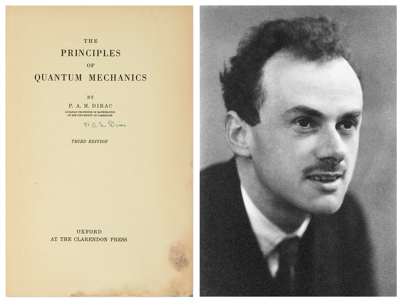
Paul Dirac

The story is similar when considering the work of Paul Dirac (1902–1984), the legendary and enigmatic physicist for whom the delta function was eventually named. The concept given by properties (1)-(3) is first defined using the delta notation in his groundbreaking Principles of Quantum Mechanics, wherein the theoretical principles of the quantum theory of matter were written in monograph form for the first time. Dirac uses the delta function in this context to define the coefficients of the orthonormal eigenfunctions for a system with a continuous spectrum of eigenvalues. Dirac used the δ notation since this is the continuous analog of a discrete operator known already as the Kronecker delta.

Without digging any further in the the dirty details of the mathematics
of quantum mechanics, it suffices to say that Dirac’s theory was criticized as
lacking rigor by mathematicians for reasons intimately related to how the delta function is not a function. Furthermore, Dirac appears to be fully aware of this issue, and can be seen trying to get ahead of his accusers. To quote from the first edition of his work [3]:

The introduction of the δ function into our analysis will not be in
itself a source of lack of rigour in the theory…The δ function in
thus merely a convenient notation. The only lack of rigour in the
theory arises from the fact that we perform operations on the abstract symbols, such as differentiation and integration with respect
to parameters occurring in them, which are not rigorously defined.
When these operations are permissible, the δ function may be used
freely for dealing with the representatives of the abstract symbols,
as though it were a continuous function, without leading to incorrect
results.

It is thus clear that Dirac was aware of his mathematical sins. Like Heaviside, Dirac was completely willing to use ill-defined symbolic tools to achieve incredible, useful, practical results. For the former these were the solutions to a wide and general class of problems in electrical engineering; for Dirac, his results were nothing less than the foundations of modern physics.

But Dirac’s reflections on his own theory probe directly into the heart of
considerations leading to the work which removes all ambiguity from the delta function and provides the mathematical rigor he knew was lacking. Started by Sergei Sobolev (1908–1989) and rendered in a polished form by Laurent Schwartz (1915–2002), this work would transform and generalize our theory of functions, differentiation, and mathematical analysis. This is the so-called theory of Distributions, or Generalized Functions.

Distributions

The core issue at the heart of the troubles with the Dirac delta and similar
mathematical objects is the problem of differentiability. As Dirac stated in the quotation above, you don’t really run in to trouble if you use his δ function as a symbolic rule for how it acts on other functions; however, he proceeds to differentiate δ in his calculations, and this is where the problems really start. How can one know a priori “when these operations are permissible” when one does not even have a firm definition of the objects, or what it would mean to differentiate them? We will see how these questions lead to the derivation of new and rigorously defined mathematical objects.

Functionals

Consider how one normally determines the derivative (or antiderivative) of a function. Under normal circumstances, with “classical” functions, you have a well-defined rule that describes how a function maps one set of real numbers to another set, say f : ℝ →ℝ. Given this and the definitions of the integral or derivative, one can then plainly investigate the values that these operators yield when applied to the function. In the case of δ, we have no workable definition to proceed along these lines. Instead, in practice δ is most prominently defined by how it operates on other, well defined functions (as in (3)). This is the key insight that leads to the modern theory of distributions. It turns out that the correct way to mathematically treat δ, and a large class of similar objects, is to stop trying to define them as functions at all. This line of thought is well described by Jean Dieudonne in his review of [4] (see [5]):

… one starts with a family of very “regular” functions (usually with
respect to differential properties), which satisfy certain (generally
integral) relations, or on which certain operations are possible; and
then one discovers that an a priori larger family of functions satisfies
the same relations, or can be subjected to similar operations. Many
questions then may naturally be asked: Is this new family really
different from the first? If it is, what are the relations between the
two families, and can one give a precise description of the new one?
It is only in the last stage of the “prehistory” that what may be
called a revolutionary point of view will emerge, with the idea that
the “new family” might consist of objects other than functions.

The other objects alluded to are functionals. You can think of a functional
as a function of functions. As a function is a unique mapping from one set of
numbers to another, a functional F can be defined as a mapping F : C →ℝ,
where C is some set of functions. That is, a functional maps functions to real
numbers. A simple example of a functional of this type is the definite integral:

which clearly takes a function f from some set of suitably integrable functions and maps it to a real number, the value of the integral, or the area under the curve f(x)between a and b. This is just a single example. One can imagine an infinite number of functionals, and sets of functionals; one could even continue to generalize and define mappings from sets of functionals to real numbers. That is neither here nor there. What is important is that the functional concept can be used to define distributions.

The Set of Test Functions

We require one more definition in order to achieve our goal. This amounts to specifying the set C of functions from which the distributions will map functions to real numbers. Functions are often collected in sets which specify their degree of continuity, differentiability, and the continuity of their derivatives. We say a function f is in the set C⁰ (write f ∈ C⁰) if it is continuous over the whole real line in the sense that the limit at all points is the same when taken from the left or the right; it is not necessarily differentiable. We say that f ∈ C¹ if its derivative does exist and is continuous, i.e. f ’ ∈ C⁰. For example, the function g(x) = |x| is continuous but not differentiable at x= 0; g is in C⁰ but not in C¹. We can generalize this and say that Cⁿ is the set of functions which have for continuous functions their first n derivatives, where n is an integer.

As n becomes larger, the sets become in a sense “smaller;” you can always find functions (infinitely many!) that are in Cⁿ but not Cⁿ⁺¹. These “continuity spaces” therefore form a sequence of nested subsets, as depicted below.

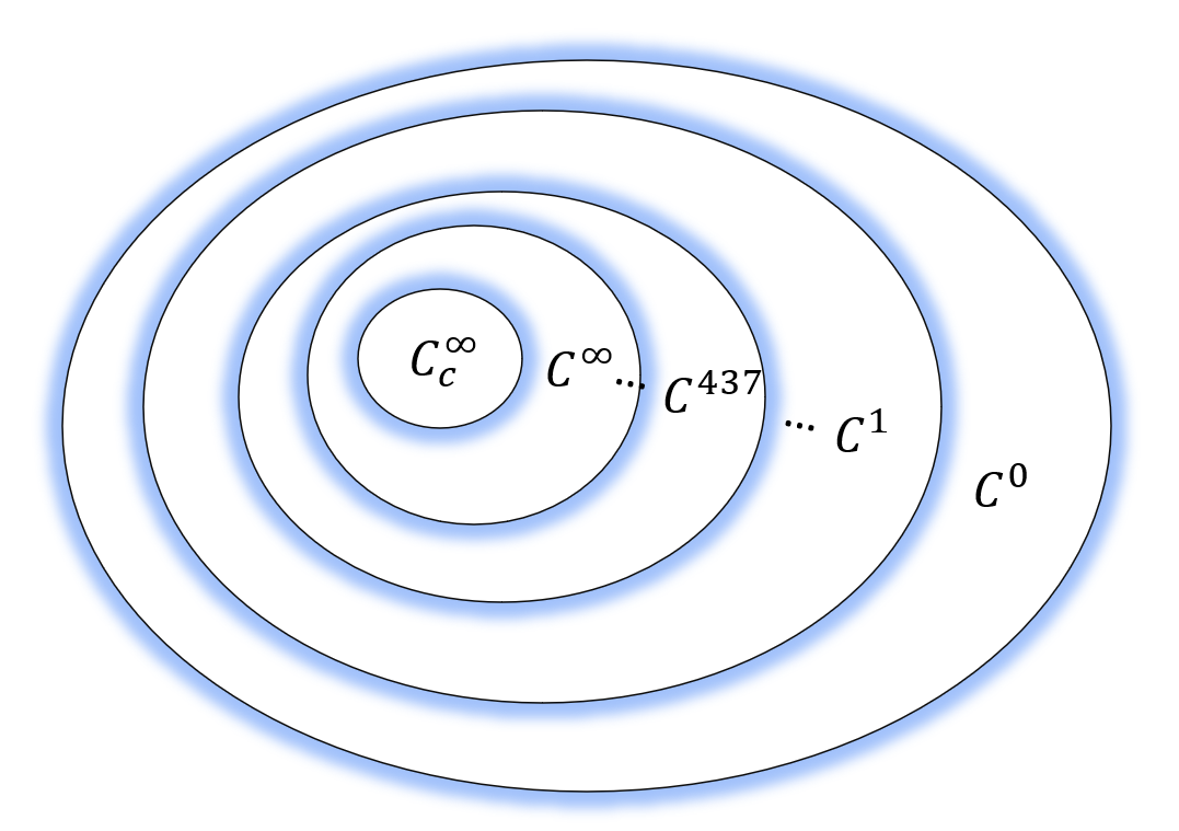
Near the bottom of this infinite sequence of sets of functions we find the set

which is of course the set of all functions which have infinitely many continuous derivatives. Many well-known and friendly functions are in this latter class (e.g. sin(x); cos(x); eˣ; all polynomials). These functions are called “smooth” or “well behaved” because one can perform the operation of differentiation on them as many time as one pleases without care. But while this set certainly has infinitely many members, they are rare in the sense that most functions are not so well behaved.

The set which is suitable for the definition of distributions is even smaller
than this. It requires an additional criterion: that the functions have compact support. This technical term means simply that a function has nonzero values within a finite domain, and is uniformly zero outside of this. We therefore use the notation

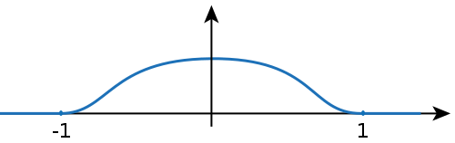
to denote the set of infinitely continuously differentiable functions with compact support, and call such functions test functions. In order to define a class of functionals using this set as a domain, we should be sure that there are actually members of this set. One example is the so-called bump function,

Feel free to verify that the bump function is a test function via differentiation. In fact there are uncountably infinitely many test functions.

The bump function, an archetypal test function.

The Definition

From this point the definition of a distribution is straightforward. A distribution is a linear functional

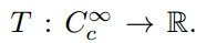
That is, it is a mapping from the set of test functions to a real number. Analogous to how a specific function acts on an input number and produces an output, specific distributions are defined by how they transform test functions into numbers. The distribution acting of test function φ can be written as T (φ), or commonly as〈T,φ〉.

One can now see why distributions are called generalized functions. For any
classical function for which the integral

is well defined, there is a corresponding distribution F such that 〈F,φ〉gives the value of this integral. However, there are also distributions which do not correspond with classical functions; distributions are more general. As should be clear by now, the canonical example of a distribution which does not correspond to a classical function is the Dirac δ. We therefore finally arrive at a fully rigorous definition of δ as the distribution such that

The Generalized or “Weak” Derivative

The δ distribution is only one of infinitely many distributions which do not
correspond to classical functions. We can obtain some more of these by differentiating δ in the sense of distributions. But how does the concept of a
distribution solve the problem of differentiation as discussed earlier? We need only generalize the concept of differentiation to apply to distributions.

Consider a function f ∈ C¹, so that it is continuously differentiable. Calculating using integration by parts, we see that

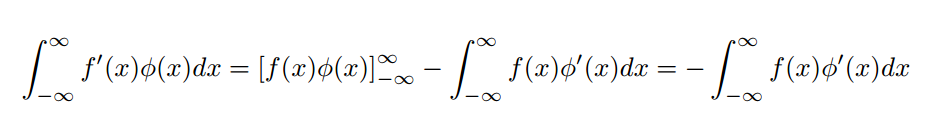
The term in the brackets vanishes since φ, as a test function, has compact support. This generalizes to a distribution, say F’, corresponding to the function f’:

This calculation generalizes quite easily to distributions that do not correspond to a classical function f. In this way, we can define the derivative T’ of T in the sense of distributions:

This is also sometimes referred to as the weak derivative, since it extends derivatives to functions which normally would not be differentiable. This generalizes even further, to higher order derivatives. We can define the nth derivative of a distribution T as T⁽ⁿ⁾, where the latter is the distribution such that

Here,

is the classical derivative of the test function, which is assured
to exist by the very definition of test functions! It follows that all distributions are infinitely differentiable (in the sense of distributions).

This removes entirely the struggle which Dirac and others faced when differentiating the δ function. By what we have defined here, a derivative of δ simply sifts for the value of another functions derivative at zero. Formally,

This provides a rigorous mathematical framework for the derivatives of δ that appeared in the literature long before this theory came into existence.

There are a number of other operations which apply to functions which have been generalized to apply to distributions. They can be added and subtracted, convolved, and transformed using Laplace and Fourier transforms. However, it is impossible to define the multiplication of distributions in a way that preserves the algebra that applies to classical functions (The Schwartz Impossibility Theorem).