Dijkstra’s Shortest Path Algorithm in Python

From GPS navigation to network-layer link-state routing, Dijkstra’s Algorithm powers some of the most taken-for-granted modern services. Utilizing some basic data structures, let’s get an understanding of what it does, how it accomplishes its goal, and how to implement it in Python (first naively, and then with good asymptotic runtime!)

What does it do?

Dijkstra’s Algorithm finds the shortest path between two nodes of a graph. So, if we have a mathematical problem we can model with a graph, we can find the shortest path between our nodes with Dijkstra’s Algorithm.

Let’s Make a Graph

First things first. A graph is a collection of nodes connected by edges:

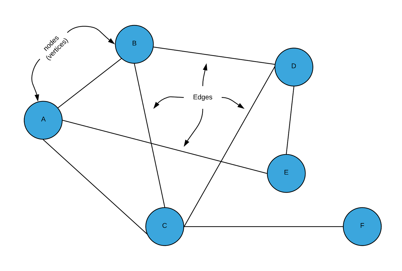
A node is just some object, and an edge is a connection between two nodes. Depicted above an undirected graph, which means that the edges are bidirectional. There also exist directed graphs, in which each edge also holds a direction.

Both nodes and edges can hold information. For example, if this graph represented a set of buildings connected by tunnels, the nodes would hold the information of the name of the building (e.g. the string “Library”), and the edges could hold information such as the length of the tunnel.

Graphs have many relevant applications: web pages (nodes) with links to other pages (edges), packet routing in networks, social media networks, street mapping applications, modeling molecular bonds, and other areas in mathematics, linguistics, sociology, and really any use case where your system has interconnected objects.

Graph Implementation

This step is slightly beyond the scope of this article, so I won’t get too far into the details. The two most common ways to implement a graph is with an adjacency matrix or adjacency list. Each has their own sets of strengths and weaknesses. I will be showing an implementation of an adjacency matrix at first because, in my opinion, it is slightly more intuitive and easier to visualize, and it will, later on, show us some insight into why the evaluation of our underlying implementations have a significant impact on runtime. Either implementation can be used with Dijkstra’s Algorithm, and all that matters for right now is understanding the API, aka the abstractions (methods), that we can use to interact with the graph. Let’s quickly review the implementation of an adjacency matrix and introduce some Python code. If you want to learn more about implementing an adjacency list, this is a good starting point.

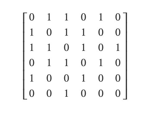
Below is the adjacency matrix of the graph depicted above. Each row is associated with a single node from the graph, as is each column. In our case, row 0 and column 0 will be associated with node “A”; row 1 and column 1 with node “B”, row 3 and column 3 with “C”, and so on. Each element at location {row, column} represents an edge. As such, each row shows the relationship between a single node and all other nodes. A “0” element indicates the lack of an edge, while a “1” indicates the presence of an edge connecting the row_node and the column_node in the direction of row_node → column_node. Because the graph in our example is undirected, you will notice that this matrix is equal to its transpose (i.e. it is a symmetric matrix) because each connection is bidirectional. You will also notice that the main diagonal of the matrix is all 0s because no node is connected to itself. In this way, the space complexity of this representation is wasteful.

Now let’s see some code. Note that I am doing a little extra — since I wanted actual node objects to hold data for me I implemented an array of node objects in my Graphclass whose indices correspond to their row (column) number in the adjacency matrix. I also have a helper method in Graph that allows me to use either a node’s index number or the node object as arguments to my Graph’s methods. These classes may not be the most elegant, but they get the job done and make working with them relatively easy:

I can use these Node and Graph classes to describe our example graph. We can set up our graph above in code and see that we get the correct adjacency matrix:

Our output adjacency matrix (from graph.print_adj_mat())when we run this code is exactly the same as we calculated before:

[0, 1, 1, 0, 1, 0]
[1, 0, 1, 1, 0, 0]
[1, 1, 0, 1, 0, 1]
[0, 1, 1, 0, 1, 0]
[1, 0, 0, 1, 0, 0]
[0, 0, 1, 0, 0, 0]

If I wanted to add some distances to my graph edges, all I would have to do is replace the 1s in my adjacency matrix with the value of the distance. Currently, myGraph class supports this functionality, and you can see this in the code below. I will add arbitrary lengths to demonstrate this:

Which outputs the adjacency matrix:

[0 , 5 , 10, 0, 2, 0]
[5 , 0 , 2 , 4 , 0 , 0]
[10, 2, 0, 7, 0, 10]
[0 , 4 , 7 , 0 , 3 , 0]
[2 , 0 , 0 , 3 , 0 , 0]
[0, 0 , 10, 0 , 0 , 0]

And visually, our graph would now look like this:

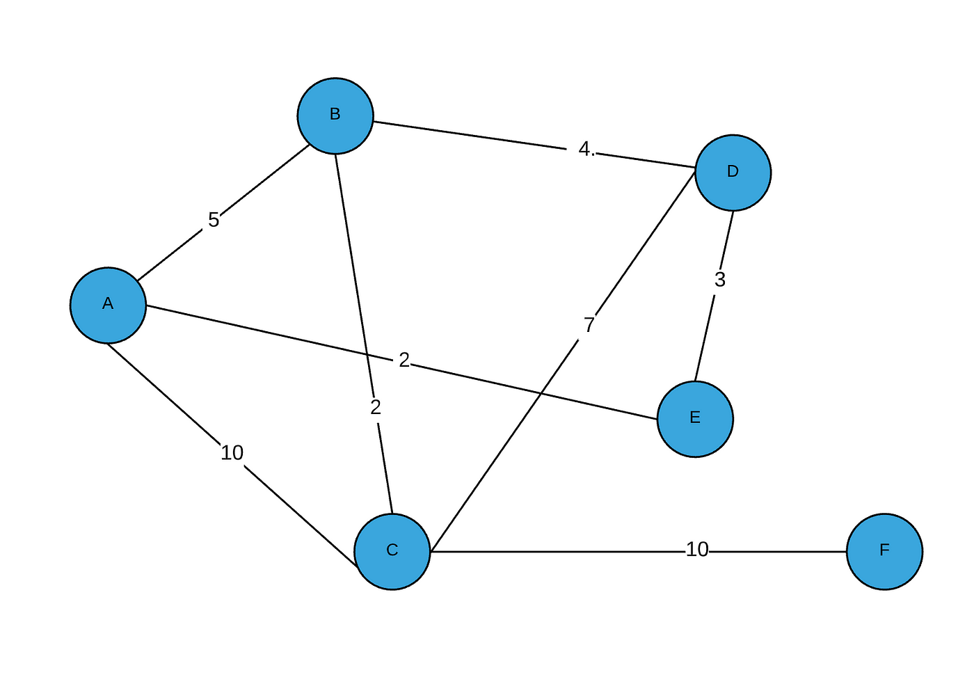
If I wanted my edges to hold more data, I could have the adjacency matrix hold edge objects instead of just integers.

Dijkstra’s Algorithm, Ho!

Before we jump right into the code, let’s cover some base points.

1. Major stipulation: we can’t have negative edge lengths.
2. Dijkstra’s algorithm was originally designed to find the shortest path between 2 particular nodes. However, it is also commonly used today to find the shortest paths between a source node and all other nodes. I will be programming out the latter today. To accomplish the former, you simply need to stop the algorithm once your destination node is added to your seenset (this will make more sense later).

Ok, onto intuition. We want to find the shortest path in between a source node and all other nodes (or a destination node), but we don’t want to have to check EVERY single possible source-to-destination combination to do this, because that would take a really long time for a large graph, and we would be checking a lot of paths which we should know aren’t correct! So we decide to take a greedyapproach! You have to take advantage of the times in life when you can be greedy and it doesn’t come with bad consequences!

So what does it mean to be a greedy algorithm? It means that we make decisions based on the best choice at the time. This isn’t always the best thing to do — for example, if you were implementing a chess bot, you wouldn’t want to take the other player’s queen if it opened you up for a checkmate the next move! For situations like this, something like minimax would work better. In our case today, this greedy approach is the best thing to do and it drastically reduces the number of checks I have to do without losing accuracy. How?? Well, let’s say I am at my source node. I will assume an initial provisional distance from the source node to each other node in the graph is infinity (until I check them later). I know that by default the source node’s distance to the source node is minium (0) since there cannot be negative edge lengths. My source node looks at all of its neighbors and updates their provisional distance from the source node to be the edge length from the source node to that particular neighbor (plus 0). Note that you HAVE to check every immediate neighbor; there is no way around that. Next, my algorithm makes the greedy choice to next evaluate the node which has the shortest provisional distance to the source node. I mark my source node as visited so I don’t return to it and move to my next node. Now let’s consider where we are logically because it is an important realization. The node I am currently evaluating (the closest one to the source node) will NEVER be re-evaluated for its shortest path from the source node. Its provisional distance has now morphed into a definite distance. Even though there very well could be paths from the source node to this node through other avenues, I am certainthat they will have a higher cost than the node’s current path because I chose this node because it was the shortest distance from the source node than any other node connected to the source node. So any other path to this mode must be longer than the current source-node-distance for this node. Using our example graph, if we set our source node as A, we would set provisional distances for nodes B, C, and E. Because Ehad the shortest distance from A, we then visited node E. Now, even though there are multiple other ways to get from Ato E, I know they have higher weights than my current A→ E distance because those other routes must go through Bor C, which I have verified to be farther from Athan E is from A. My greedy choice was made which limits the total number of checks I have to do, and I don’t lose accuracy! Pretty cool.

Continuing the logic using our example graph, I just do the same thing from E as I did from A. I update all of E's immediate neighbors with provisional distances equal to length(A to E) + edge_length(E to neighbor) IF that distance is less than it’s current provisional distance, or a provisional distance has not been set. (Note: I simply initialize all provisional distances to infinity to get this functionality). I then make my greedy choice of what node should be evaluated next by choosing the one in the entire graph with the smallest provisional distance, and add E to my set of seen nodes so I don’t re-evaluate it. This new node has the same guarantee as E that its provisional distance from A is its definite minimal distance from A. To understand this, let’s evaluate the possibilities (although they may not correlate to our example graph, we will continue the node names for clarity). If the next node is a neighbor of E but not of A, then it will have been chosen because its provisional distance is still shorter than any other direct neighbor of A, so there is no possible other shortest path to it other than through E. If the next node chosen IS a direct neighbor of A, then there is a chance that this node provides a shorter path to some of E's neighbors than E itself does.

Algorithm Overview

Now let’s be a little more formal and thorough in our description.

INITIALIZATION

1. Set the provisional_distance of all nodes from the source node to infinity.
2. Define an empty set of seen_nodes. This set will ensure we don’t re-evaluate a node which already has the shortest path set, and that we don’t evaluate paths through a node which has a shorter path to the source than the current path. Remember that nodes only go into seen_nodes once we are sure that we have their absolute shortest distance (not just their provisional distance). We use a set so that we get that sweet O(1) lookup time rather than repeatedly searching through an array at O(n) time.
3. Set the provisional_distance of the source node to equal 0, and the array representing the hops taken to just include the source node itself. (This will be useful later as we track which path through the graph we take to get the calculated minimum distance).

ITERATIVE PROCEDURE

4. While we have not seen all nodes (or, in the case of source to single destination node evaluation, while we have not seen the destination node):

5. Set current_node to the node with the smallest provisional_distance in the entire graph. Note that for the first iteration, this will be the source_nodebecause we set its provisional_distance to 0.

6. Add current_node to the seen_nodes set.

7. Update the provisional_distance of each of current_node's neighbors to be the (absolute) distance from current_node to source_node plus the edge length from current_node to that neighbor IF that value is less than the neighbor’s current provisional_distance. If this neighbor has never had a provisional distance set, remember that it is initialized to infinity and thus must be larger than this sum. If we update provisional_distance, also update the “hops” we took to get this distance by concatenating current_node's hops to the source node with current_node itself.

8. End While.

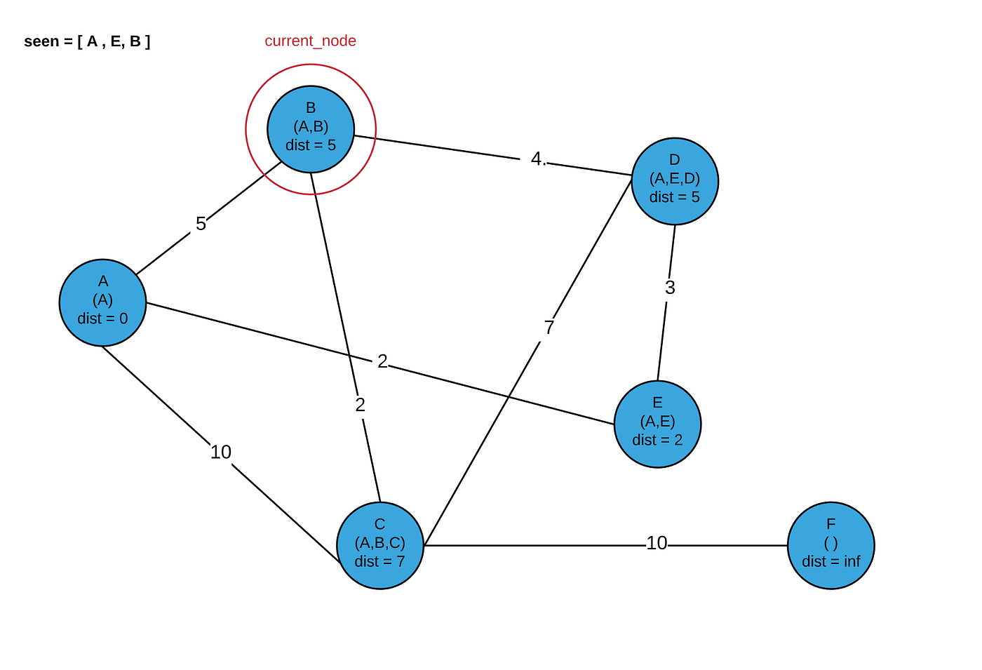
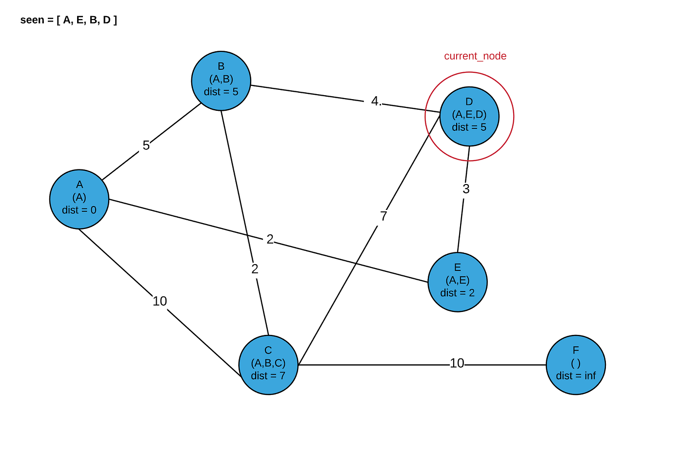
With Pictures

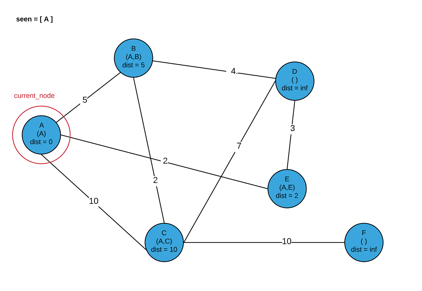
Note that next, we could either visit D or B. I will choose to visit B.

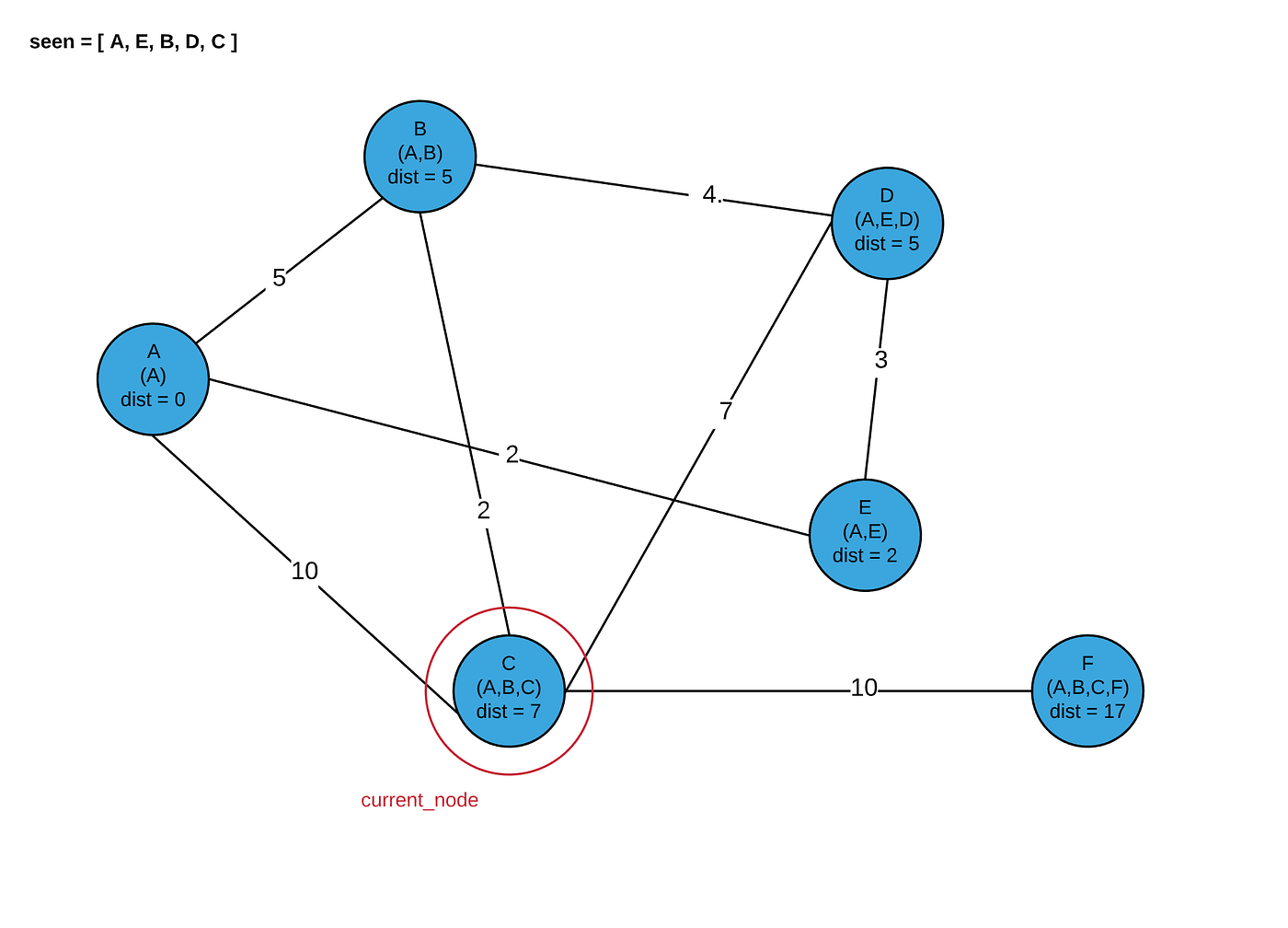
Now our program terminates, and we have the shortest distances and paths for every node in our graph!

It’s Time To Code

Let’s see what this may look like in python (this will be an instance method inside our previously coded Graph class and will take advantage of its other methods and structure):

We can test our picture above using this method:

To get some human-readable output, we map our node objects to their data, which gives us the output:

[(0, [‘A’]), (5, [‘A’, ‘B’]), (7, [‘A’, ‘B’, ‘C’]), (5, [‘A’, ‘E’, ‘D’]), (2, [‘A’, ‘E’]), (17, [‘A’, ‘B’, ‘C’, ‘F’])]

Where each tuple is (total_distance, [hop_path]). This matches our picture above!

Cool! Are We Done?

Nope! But why? We can make this faster! If all you want is functionality, you are done at this point!

For the brave of heart, let’s focus on one particular step. Each iteration, we have to find the node with the smallest provisional distance in order to make our next greedy decision. Right now, we are searching through a list we calledqueue(using the values in dist) in order to find what we need. This queue can have a maximum length n, which is our number of nodes. Our iteration through this list, therefore, is an O(n) operation, which we perform every iteration of our while loop. Since our while loop runs until every node is seen, we are now doing an O(n) operation n times! So our algorithm is O(n²)!! That isn’t good. But that’s not all! If you look at the adjacency matrix implementation of our Graph, you will notice that we have to look through an entire row (of size n) to find our connections! That is another O(n) operation in our while loop. How can we fix it? Well, first we can use a heap to get our smallest provisional distance in O(lg(n)) time instead of O(n) time (with a binary heap — note that a Fibonacci heap can do it in O(1)), and second we can implement our graph with an Adjacency List, where each node has a list of connected nodes rather than having to look through all nodes to see if a connection exists. This shows why it is so important to understand how we are representing data structures. If we implemented a heap with an Adjacency Matrix representation, we would not be changing the asymptotic runtime of our algorithm by using a heap! (Note: If you don’t know what big-O notation is, check out my blog on it!)

Heaps

So there are these things called heaps. We commonly use them to implement priority queues. Basically what they do is efficiently handle situations when we want to get the “highest priority” item quickly. For us, the high priority item is the smallest provisional distance of our remaining unseen nodes. Instead of searching through an entire array to find our smallest provisional distance each time, we can use a heap which is sitting there ready to hand us our node with the smallest provisional distance. Once we take it from our heap, our heap will quickly re-arrange itself so it is ready to hand us our next value when we need it. Pretty cool! If you want to challenge yourself, you can try to implement the really fast Fibonacci Heap, but today we are going to be implementing a Binary MinHeap to suit our needs.

A binary heap, formally, is a complete binary tree that maintains the heap property. Ok, sounds great, but what does that mean?

Complete Binary Tree: This is a tree data structure where EVERY parent node has exactly two child nodes. If there are not enough child nodes to give the final row of parent nodes 2 children each, the child nodes will fill in from left to right.

What does this look like?

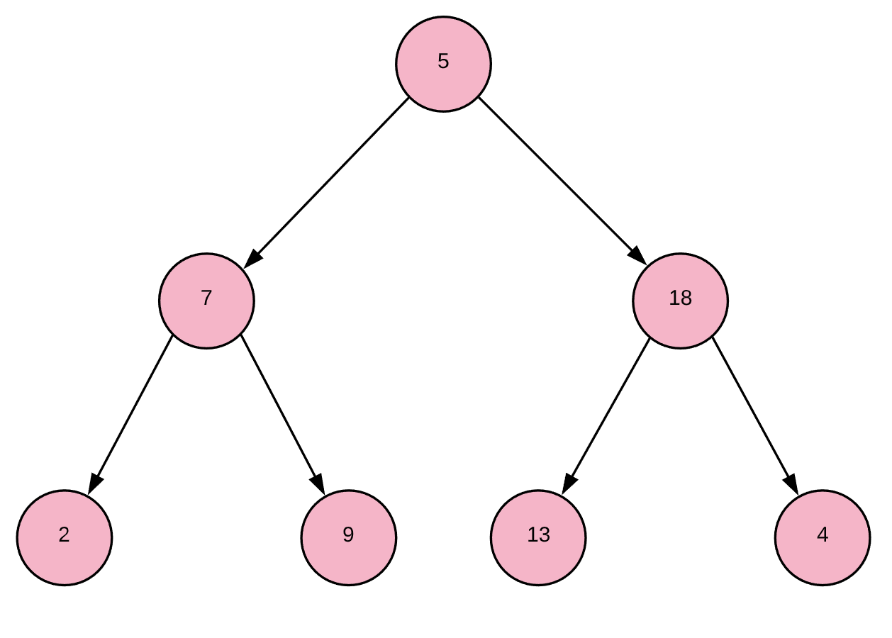
The Heap Property: (For a Minimum Heap) Every parent MUST be less than or equal to both of its children.

Applying this principle to our above complete binary tree, we would get something like this:

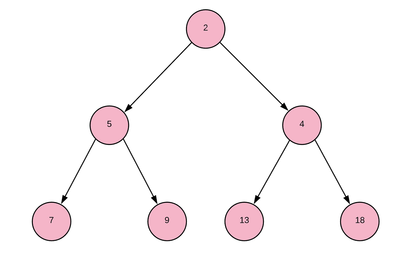
Which would have the underlying array [2,5,4,7,9,13,18]. As you can see, this is semi-sorted but does not need to be fully sorted to satisfy the heap property. This “underlying array” will make more sense in a minute.

Now we know what a heap is, let’s program it out, and then we will look at what extra methods we need to give it to be able to perform the actions we need it to!

So, we know that a binary heap is a special implementation of a binary tree, so let’s start out by programming out a BinaryTreeclass, and we can have our heap inherit from it. To implement a binary tree, we will have our underlying data structure be an array, and we will calculate the structure of the tree by the indices of our nodes inside the array. For example, our initial binary tree (first picture in the complete binary tree section) would have an underlying array of [5,7,18,2,9,13,4]. We will determine relationships between nodes by evaluating the indices of the node in our underlying array. Since we know that each parent has exactly 2 children nodes, we call our 0th index the root, and its left child can be index 1 and its right child can be index 2. More generally, a node at index iwill have a left child at index 2*i + 1 and a right child at index 2*i + 2. A node at indexi will have a parent at index floor((i-1) / 2).

So, our BinaryTree class may look something like this:

Now, we can have our MinHeap inherit from BinaryTree to capture this functionality, and now our BinaryTree is reusable in other contexts!

Alright, almost done! Now all we have to do is identify the abilities our MinHeapclass should have and implement them! We need our heap to be able to:

• Turn itself from an unordered binary tree into a minimum heap. This will be done upon the instantiation of the heap.
• Pop off its minimum value to us and then restructure itself to maintain the heap property. This will be used when we want to visit our next node.
• Update (decrease the value of) a node’s value while maintaining the heap property. This will be used when updating provisional distances.

To accomplish these, we will start with a building-block which will be instrumental to implement the first two functions. Let’s write a method called min_heapify_subtree. This method will assume that the entire heap is heapified(i.e. satisfying the heap property) except for a single 3-node subtree. We will heapify this subtree recursively by identifying its parent node index at i and allowing the potentially out-of-place node to be placed correctly in the heap. To do this, we check to see if the children are smaller than the parent node and if they are we swap the smallest child with the parent node. Then, we recursively call our method at the index of the swapped parent (which is now a child) to make sure it gets put in a position to maintain the heap property. Here’s the pseudocode:

FUNCTION min_heapify_subtree(i)
index_of_min = i
IF left_child exists AND left_child < node[index_of_min]
index_of_min = left_child_index
ENDIF
IF right_child exists AND right_child < node[index_of_min]
index_of_min = right_child_index
ENDIF
IF index_of_min != i
swap(nodes[i], nodes[index_of_min])
min_heapify_subtree(index_of_min)
ENDIF
END

In the worst-case scenario, this method starts out with index 0 and recursively propagates the root node all the way to the bottom leaf. Because our heap is a binary tree, we have lg(n) levels, where n is the total number of nodes. Because each recursion of our method performs a fixed number of operations, i.e. is O(1), we can call classify the runtime of min_heapify_subtree to be O(lg(n)).

To turn a completely random array into a proper heap, we just need to call min_heapify_subtree on every node, starting at the bottom leaves. So, we can make a method min_heapify:

FUNCTION min_heapify
FOR index from last_index to first_index
min_heapify_subtree(index)
ENDFOR
END

This method performs an O(lg(n)) method n times, so it will have runtime O(nlg(n)).

We will need to be able to grab the minimum value from our heap. We can read this value in O(1) time because it will always be the root node of our minimum heap (i.e. index 0 of the underlying array), but we want to do more than read it. We want to remove it AND then make sure our heap remains heapified. To do that, we remove our root node and replace it by the last leaf, and then min_heapify_subtree at index 0 to ensure our heap property is maintained:

FUNCTION pop
min_node = nodes[0]
IF heap_size > 1
nodes[0] = nodes[nodes.length - 1]
nodes.pop() // remove the last element from our nodes array
min_heapify_subtree(0)
ELSE IF heap_size == 1
nodes.pop()
ELSE
return NIL // the heap is empty, so return NIL value
ENDIF
return min_node
END

Because this method runs in constant time except for min_heapify_subtree, we can say this method is also O(lg(n)).

Great! Now for our last method, we want to be able to update our heap’s values (lower them, since we are only ever updating our provisional distances to lower values) while maintaining the heap property!

So, we will make a method called decrease_key which accepts an index value of the node to be updated and the new value. We want to update that node’s value, and then bubble it up to where it needs to be if it has become smaller than its parent! So, until it is no longer smaller than its parent node, we will swap it with its parent node:

FUNCTION decrease_key(index, value)
nodes[index] = value
parent_node_index = parent_index(index)
WHILE index != 0 AND nodes[parent_node_index] > nodes[index]
swap(nodes[i], nodes[parent_node_index])
index = parent_node_index
parent_node_index = parent_index(index)
ENDWHILE
END

Ok, let’s see what all this looks like in python!

Whew! Ok, time for the last step, I promise! We just have to figure out how to implement this MinHeap data structure into our dijsktra method in our Graph, which now has to be implemented with an adjacency list. We want to implement it while fully utilizing the runtime advantages our heap gives us while maintaining our MinHeap class as flexible as possible for future reuse!

So first let’s get this adjacency list implementation out of the way. Instead of a matrix representing our connections between nodes, we want each node to correspond to a list of nodes to which it is connected. This way, if we are iterating through a node’s connections, we don’t have to check ALL nodes to see which ones are connected — only the connected nodes are in that node’s list. So, our old graph friend

would have the adjacency list which would look a little like this:

[
[ NodeA, [(NodeB, 5), (NodeC, 10), (NodeE, 2)] ],
[ NodeB, [(NodeA, 5), (NodeC, 2), (NodeD, 4)] ],
[ NodeC, [(NodeA, 10), (NodeB, 2), (NodeD, 7), (NodeF, 10)] ],
[ NodeD, [(NodeB, 4), (NodeC, 7), (NodeE, 3)] ],
[ NodeE, [(NodeA, 2), (NodeD, 3)] ],
[ NodeF, [(NodeC, 10)]
]

As you can see, to get a specific node’s connections we no longer have to evaluate ALL other nodes. Let’s keep our API as relatively similar, but for the sake of clarity we can keep this class lighter-weight:

Next, let’s focus on how we implement our heap to achieve a better algorithm than our current O(n²) algorithm. If we look back at our dijsktra method in our Adjacency Matrix implementedGraph class, we see that we are iterating through our entire queue to find our minimum provisional distance (O(n) runtime), using that minimum-valued node to set our current node we are visiting, and then iterating through all of that node’s connections and resetting their provisional distance as necessary (check out the connections_to or connections_from method; you will see that it has O(n) runtime). These two O(n) algorithms reduce to a runtime of O(n) because O(2n) = O(n). We are doing this for every node in our graph, so we are doing an O(n) algorithm n times, thus giving us our O(n²) runtime. Instead, we want to reduce the runtime to O((n+e)lg(n)), where n is the number of nodes and e is the number of edges.

In our adjacency list implementation, our outer while loop still needs to iterate through all of the nodes (n iterations), but to get the edges for our current node, our inner loop just has to iterate through ONLY the edges for that specific node. Thus, that inner loop iterating over a node’s edges will run a total of only O(n+e) times. Inside that inner loop, we need to update our provisional distance for potentially each one of those connected nodes. This will utilize the decrease_keymethod of our heap to do this, which we have already shown to be O(lg(n)). Thus, our total runtime will be O((n+e)lg(n)).

New algorithm:

INITIALIZATION

1. Set the provisional_distance of all nodes from the source node to infinity except for our source node, which will be set to 0. And add this data to a minimum heap.
2. Instead of keeping a seen_nodes set, we will determine if we have visited a node or not based on whether or not it remains in our heap. Remember when we pop() a node from our heap, it gets removed from our heap and therefore is equivalent in logic to having been “seen”.

ITERATIVE PROCEDURE

3. While the size of our heap is > 0: (runs n times)

4. Set current_node to the return value of heap.pop().

5. For n in current_node.connections, use heap.decrease_key if that connection is still in the heap (has not been seen) AND if the current value of the provisional distance is greater than current_node's provisional distance plus the edge weight to that neighbor. This for loop will run a total of n+e times, and its complexity is O(lg(n)).

6. End While.

There are 2 problems we have to overcome when we implement this:

Problem 1: We programmed our heap to work with an array of numbers, but we need our heap’s nodes to encapsulate the provisional distance (the metric to which we heapify), the hops taken, AND the node which that distance corresponds to.

Problem 2: We have to check to see if a node is in our heap, AND we have to update its provisional distance by using the decrease_key method, which requires the index of that node in the heap. But our heap keeps swapping its indices to maintain the heap property! We have to make sure we don’t solve this problem by just searching through our whole heap for the location of this node. This would be an O(n) operation performed (n+e) times, which would mean we made a heap and switched to an adjacency list implementation for nothing! We need to be able to do this in O(1) time.

Solution 1: We want to keep our heap implementation as flexible as possible. To allow it to accept any data type as elements in the underlying array, we can just accept optional anonymous functions (i.e. lambdas) upon instantiation, which are provided by the user to specify how it should deal with the elements inside the array should those elements be more complex than just a number. The default value of these lambdas could be functions that work if the elements of the array are just numbers. So, if a plain heap of numbers is required, no lambdas need to be inserted by the user. We will need these customized procedures for comparison between elements as well as for the ability to decrease the value of an element. We can call our comparison lambda is_less_than, and it should default to lambda: a,b: a < b. Our lambda to return an updated node with a new value can be called update_node, and it should default simply to lambda node, newval: newval. By passing in the node and the new value, I give the user the opportunity to define a lambda which updates an existing object OR replaces the value which is there. In the context of our oldGraph implementation, since our nodes would have had the values

[ provisional_distance, [nodes, in, hop, path]] , our is_less_than lambda could have looked like this: lambda a,b: a[0] < b[0], and we could keep the second lambda at its default value and pass in the nested array ourselves into decrease_key. However, we will see shortly that we are going to make the solution cleaner by making custom node objects to pass into our MinHeap. The flexibility we just spoke of will allow us to create this more elegant solution easily. Specifically, you will see in the code below that my is_less_than lambda becomes: lambda a,b: a.prov_dist < b.prov_dist, and my update_node lambda is: lambda node, data: node.update_data(data), which I would argue is much cleaner than if I continued to use nested arrays.

Solution 2: There are a few ways to solve this problem, but let’s try to choose one that goes hand in hand with Solution 1. Given the flexibility we provided ourselves in Solution 1, we can continue using that strategy to implement a complementing solution here. We can implement an extra array inside our MinHeap class which maps the original order of the inserted nodes to their current order inside of the nodes array. Let’s call this list order_mapping. By maintaining this list, we can get any node from our heap in O(1) time given that we know the original order that node was inserted into the heap. So, if the order of nodes I instantiate my heap with matches the index number of my Graph's nodes, I now have a mapping from my Graph node to that node’s relative location in my MinHeap in constant time! To be able to keep this mapping up to date in O(1) time, the whatever elements passed into the MinHeap as nodes must somehow “know” their original index, and my MinHeap needs to know how to read that original index from those nodes. This is necessary so it can update the value of order_mapping at the index number of the node’s index property to the value of that node’s current position in MinHeap's node list. Because we want to allow someone to use MinHeap that does not need this mapping AND we want to allow any type of data to be nodes of our heap, we can again allow a lambda to be added by the user which tells our MinHeap how to get the index number from whatever type of data is inserted into our heap — we will call this get_index. For example, if the data for each element in our heap was a list of structure [data, index], our get_index lambda would be: lambda el: el[1]. Furthermore, we can set get_index's default value to None, and use that as a decision-maker whether or not to maintain the order_mapping array. That way, if the user does not enter a lambda to tell the heap how to get the index from an element, the heap will not keep track of the order_mapping, thus allowing a user to use a heap with just basic data types like integers without this functionality. The get_indexlambda we will end up using, since we will be using a custom node object, will be very simple: lambda node: node.index().

Combining solutions 1 and 2, we will make a clean solution by making a DijkstraNodeDecorator class to decorate all of the nodes that make up our graph. This decorator will provide the additional data of provisional distance(initialized to infinity) and hops list (initialized to an empty array). Also, it will be implemented with a method which will allow the object to update itself, which we can work nicely into the lambda for decrease_key. DijkstraNodeDecoratorwill be able to access the index of the node it is decorating, and we will utilize this fact when we tell the heap how to get the node’s index using the get_indexlambda from Solution 2.

And finally, the code:

This final code, when run, outputs:

[(0, [‘a’]), (2, [‘a’, ‘e’]), (5, [‘a’, ‘e’, ‘d’]), (5, [‘a’, ‘b’]), (7, [‘a’, ‘b’, ‘c’]), (17, [‘a’, ‘b’, ‘c’, ‘f’])]

As we can see, this matches our previous output! And the code looks much nicer! AND, most importantly, we have now successfully implemented Dijkstra’s Algorithm in O((n+e)lg(n)) time!