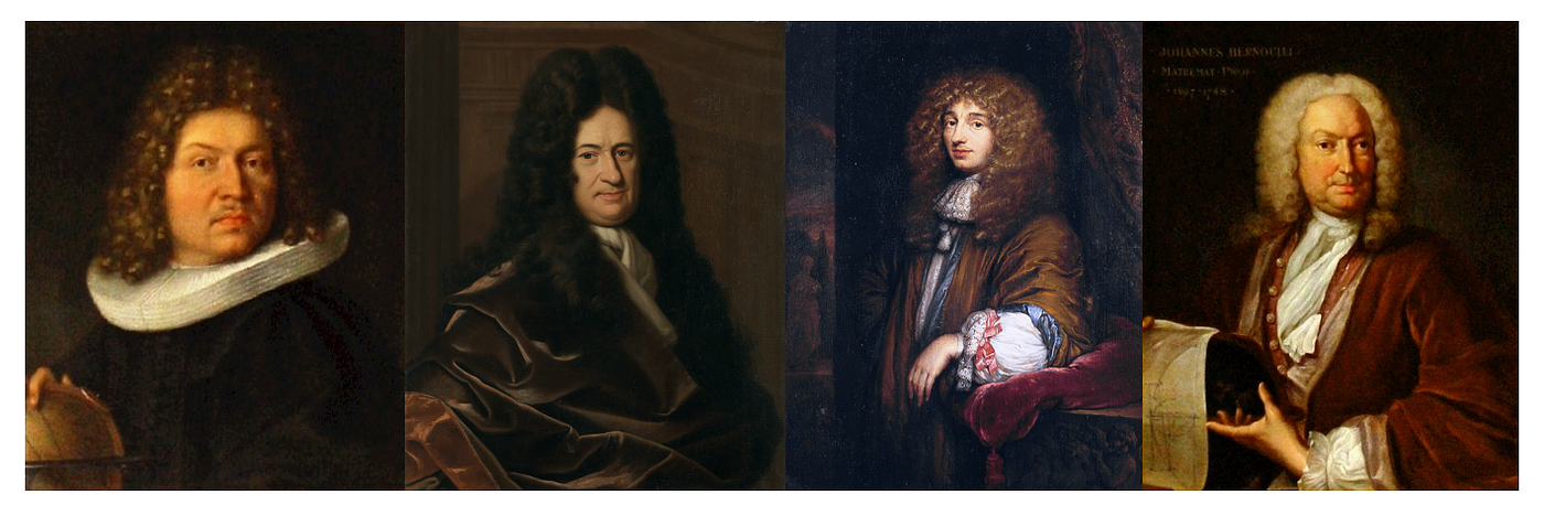
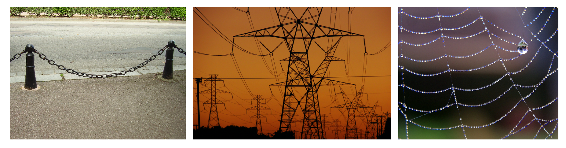
A perfectly flexible chain in equilibrium suspended by its ends and subject to gravity has the shape of a curve called the catenary. The name was coined in 1690 by the Dutch physicist, mathematician, astronomer, and inventor, Christiaan Huygens in a letter to the prominent German polymath Gottfried Leibniz.

The catenary is similar to a parabola which led the great Italian astronomer, physicist, and engineer, Galileo Galilei, the first to study it, to mistakenly identify its shape as a parabola. The correct shape was obtained independently by Leibniz, Huygens, and the Swiss mathematician Johann Bernoulli in 1691. All of them were responding to a challenge proposed by the Swiss mathematician Jacob Bernoulli (Johann's older brother) to obtain the equation of the “chain-curve.”

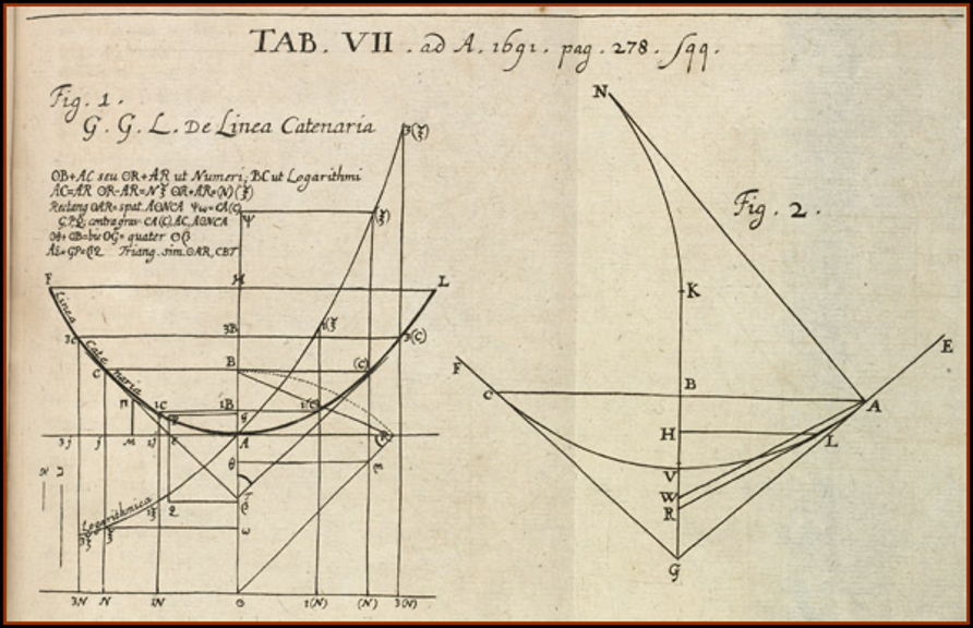
The figures that Leibniz and Huygens sent to Jacob Bernoulli are shown below. They were published in the Acta Eruditorum, the “first scientific journal of the German-speaking lands of Europe.”

Johann Bernoulli was delighted that he had successfully solved the problem his older brother Jacob failed to solve. Twenty-seven years later, he wrote in a letter:

The efforts of my brother were without success. For my part, I was more fortunate, for I found the skill (I say it without boasting; why should I conceal the truth?) to solve it in full…. It is true that it cost me study that robbed me of rest for an entire night. It was a great achievement for those days and for the slight age and experience I then had. The next morning, filled with joy, I ran to my brother, who was struggling miserably with this Gordian knot without getting anywhere, always thinking like Galileo that the catenary was a parabola. Stop! Stop! I say to him, don’t torture yourself any more try­ ing to prove the identity of the catenary with the parabola, since it is entirely false.

— Johann Bernoulli

Finding the Equation of the Catenary

To find the equation of the catenary the following assumptions are made:

• The chain (or cable) is suspended between two points and hangs under its own weight.
• The chain (or cable) is flexible and has a uniform linear weight density (equal to w₀).

The treatment here follows closely the book by Simmons. To simplify the algebra, we will let the y-axis pass through the minimum of the curve. The length of the segment from the minimum to the point (x, y) is denoted by s. The three forces acting on the segment are the tensions T₀ and T, and its weight w₀s (see figure below). The first two forces are tangent to the chain.

For the segment to be in equilibrium horizontally and vertically, the following two conditions must be obeyed:

The differential equation we need to solve is:

We now have to re-write this equation in terms of y and x only. We first differentiate it to obtain:

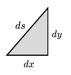
The derivative ds/dx can be written in terms of dy/dx as follows:

Eq. 3 then becomes:

To quickly solve Eq. 5 we conveniently introduce the following variable:

Using Eq. 6, Eq. 5 becomes:

This equation can be integrated by variable separation and a simple trigonometric substitution u = tan θ:

Since the y-axis pass through the minimum of the curve we have:

Substituting Eq. 9 in Eq. 8 we obtain:

Substituting c=0 into Eq. 8 and solving for u we obtain:

Thanks for reading, and see you soon! As always, constructive criticism and feedback are always welcome!

My Linkedin, personal website www.marcotavora.me, and Github have some other interesting content about math and physics and other topics such as machine learning, deep learning, finance, and much more! Check them out!