Cubic Polynomials - Using Similar Triangles to Approximate Roots

While similar triangles can be used with polynomials of any order, this introductory post is presented in cubics to exploit the compliant architecture while highlighting the practicality and simplicity of similar triangle math.

The method has particular advantages in higher order polynomials when supported by various changeable architectures, as it can alleviate onerous iterations of gradient and height calculations. This will be the subject of another post.

This post assumes math at high school level.

Similar Triangles

Similar triangles strike a chord across the x axis between points or nodes being line intercepts on the function.

The closer the nodes are together, the more accurate the cord intercept will approximate the root as shown in Diagram 1 below, where similar triangles DEFand GEH result in: approximate root G=E-Δx=E-(EH)*DF/EF) which compares with Root A, shown in red.

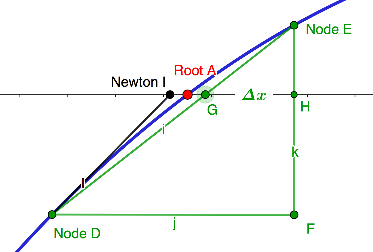
As a visual comparison, Newton’s Approximation Root I is also shown applied from Node D.

In contrast to some approximation methods, which require a single point of application like Node D above, similar triangles require two nodes D and E to straddle a target root.

These nodes can be derived ‘naturally’ as we will see with Cubic polynomials, or constructed from simultaneous equations using ‘SOSO’, a twin function with Same Opposite Same Opposite +/- coefficients.

Refer to Quintic Polynomials-Finding Roots From Primary and Secondary Nodes; a Double Shot! for an appreciation of the scope of SOSO nodes which require basic quadratic math up to Sextic order and can easily be shifted closer to a target root to provide the required two node reference coordinates for Similar Triangles. Despite the extra node, the method can require less math than other approximations, particularly with higher order functions requiring 2nd iteration gradient dy/dx, and height (y) calculations, when a root is in an area with high function concavity or convexity and/or Node(y) is relatively remote.

Natural Cubic Nodes

Cubic Polynomial symmetry offers intuitive solutions to use simple Turning Point Tp and Inflection Point Ip coordinates for natural nodederivations. When applied to cubics with 3 roots, these nodes always straddle the root with the least concave/convex root gradients, resulting in accurate one off approximations.

Example 1

Consider the following cubic function, y=2x³-3x²-3x+4 shown in blue in Graph 1 with target Root A, having the steepest gradient and least curvature of the 3 roots, and a D intercept on line Tp(y) opposing turning point F.

Everything we need from the basic architecture is shown in green.

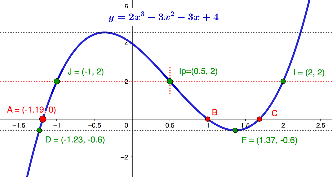
Node J

Shown is a line y=2 through the inflection point Ip=(0.5, 2) which we will use to calculate node J to become the apex of similar triangles, calculated as follows:

y=2x³-3x²-3x+4

dy/dx=6x²-6x-3 and d²y/dx²=12x-6,

Hence: Xip=0.5 from which Yip=2.

Since the sum of the factors of a cubic polynomial with 3 roots is equal to the coefficient B/A of x² similarly applies to the sum of intercepts on any line y=hwithin the range of the turning points, we can treat this as a cubic polynomial y=2x³-3x²-3x+2 and using the ‘Extended Quadratic Equation’ I presented in a post article, Cubic Polynomials-A Simpler Approach, calculate Node J as follows;

Where factor L=-0.5, which we have just found as Xip, A and B are the usual cubic coefficients and D the new constant.

Hence Root J=-1 and Root I=2 (not req’d). Hence, Node J=-1.

Node D

Node D is the intercept with the tangent y=-0.6 of Turning Point F=(1.365, -0.6) derived from dy/dx=6x²-6x-3=0 from which we can strike a chord to Node J to approximate Root A at the x axis intercept.

Again, using the sum of the factors as above we can state:

Node D(x)=-Coefficient (B/2)+2*1.365=1.5–2.74=-1.23, hence Node D=(-1.23, 0.6).

Note: Root B and Root C sum together at a turning point to equal F+0.000000….1+F-0.000000….1=2F.

Calculate Root A

A chord drawn from Node D to Node J intercepts the x axis at M, (in green) and passes very close to Root A=(-1.19, 0), (shown in red) on Diagram 2 below. It can be seen that Root A is approached closely by the hypotenuse of triangle D-J-N.

Hence Root A can be approximated by calculating Δx and adding to Node J as follows:

Δx=OJ*{D(x)-J(x)}/(OJ+ON)=-0.18, hence:

Approx. Root A=-1-0.18=-1.18 which compares with -1.19 actual.

Remaining Roots

To complete the task, the 2nd and 3rd roots are simply ‘downloaded’ from the ‘Extended Quadratic Equation’ I used above.

Where Factor L=1.18, which we have just found, A and B are usual cubic coefficients and D the constant. Hence Root B=1.02 and Root C=1.66 compared with actuals Root B=1.0 and Root C=1.69.

Summary

This post introduced similar triangles utilising basic geometry within friendly cubic polynomial architecture as an alternative root approximation method. I hope I have demonstrated its potential for wider application while adopting intuitive learning, relating the math with the graph; making math work for you; not you for it!