Using Newton’s Approximation to find the roots of polynomials is commonly taught. However, this can involve repeated iterations to achieve the required level of accuracy.

This post shows how to achieve high accuracy in a single application. The method exploits the amazing symmetry of cubic polynomials around their Inflection Point, (Xip,Yip), to find an optimal starting point for Newton’s method. I do this by exploiting polynomials’ rotational symmetry to ‘visually’ transpose a selected ‘satellite’ point on the graph to its counterpart. At these points, the gradient is steep and the concavity (second derivative) is small, so Newton’s Approximation will be accurate.

Newton’s Approximation is widely used to find a 1st root, then often followed by lengthy division or factoring to find the others. My focus here is on the 1st root, as I have previously presented a modified Quadratic Equation for finding the 2nd and 3rd roots given that the 1st is known. You can read about this in Cubic Polynomials — A Simpler Approach. I will include this method in this post for completeness.

This post assumes knowledge of algebra and introductory calculus (differentiating polynomials) at the high school level.

Newton’s Approximation

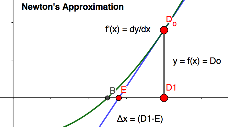
The below diagram treats a section of a curve as the ‘hypotenuse’ of a triangle, with height y=Do, and tangent angle dy/dx. The aim is to calculate point E, being an approximation to the actual root B.

With Δx=(D1-E) being the adjacent side: dy/dx=Do/Δx

Rearranging: Δx=Do/(dy/dx)

Normally the process is repeated from point E, with Δx=Eo/(dy/dx) reapplied from points E1, E2 etc., to obtain successive approximations to the root B. A stated earlier, Newton’s method will converge fast if the gradient is steep and the concavity (second derivative) is small.

Rotation to Roots

Rotation to find roots in cubic polynomials requires relatively simple calculations.

The rotation ‘satellite’ starting point x coordinate is ‘visually’ derived by adding the linear and constant terms of the cubic polynomial after neutralising the cubic and quadratic terms.

The terminal point, which is Do in the above diagram, has the same gradient as the satellite point. Meanwhile, the height Do is simply Yip-Ys, where Ys is the satellite height.

Example

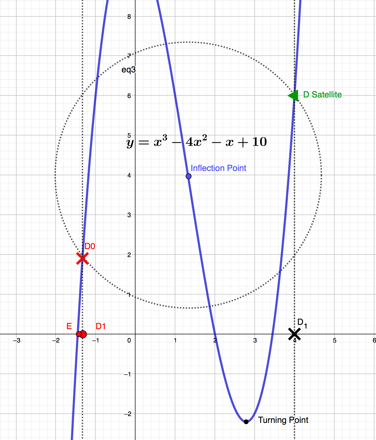
Let y=x³-4x²-x+10

Steps to Calculate Roots

A) Find the satellite point Ds by neutralising the cubic and quadratic components of the function by the value of x, and extracting the resulting sum y=Ds as follows:

Let y=x³-4x²-x+10

• When x=4, the cubic and quadratic components are equal.
• Therefore, y=6 as shown at point Ds.

B) Calculate dy/dx at point Ds:

at x=4, dy/dx=3x²-8x-1=15

C) Calculate Xip and Yip

d²y/dx²=6x-8=0

Hence: Xip=1.33,

Hence: Yip=1.33³-4*1.33²-1.33+10=3.96

D) Visually transpose Point Ds by 180 degree rotation to Do for application of Newton’s approximation and calculate height:

Do=Yip-(Ds-Yip)=3.96-(6–3.96)=1.92

E) Apply Newton’s Approximation from Do

with Δx=(D1-E) being the adjacent side: dy/dx=Do/Δx

Rearranging: Δx=Do/(dy/dx)

Δx=1.92/15=-0.128–1.33=-1.45

This compares accurately with the actual root, x=-1.45.

Note: The effectiveness of rotating to roots is maximised when the initial D1 point is outside the Xtp on the graph (as in this example) where component gradients are positive and steeper.

The right time to use it is intuitive, but larger D1 values are a positive indicator to be considered with a quick visual sketch knowing Yip, the gradient at constant D being given by the coefficient of C.

F) To complete the task, the 2nd and 3rd roots are ‘downloaded’ from the modified Quadratic Equation I posted previously.

where A=1, B=-4, C=-1 (not needed) are factors and D=+10.

Factor L, which we have just found =+1.45

Doing the math yields roots: 3.45 and 2.0, which compare with 3.45 and 2.0actuals.

This post shows that ‘Rotation to Roots’ is simple, intuitive and fast. It has limitations with functions where Ds and Yip don’t provide good D0 locations, but overall it is easy and builds an understanding of polynomial ‘architecture’. As I have shown, it can provide accurate results with a single iteration of Newton’s Approximation. But much more importantly it can help you to intuitively connect the ‘Math with the Graph’ next time you’re dealing with a polynomial.

I will explore further methods of finding the 1st root in a forthcoming post, exploiting the underlying components’ architecture.